You can access the full courses here: Build Lorenzo – A Face Swapping AI and Build Jamie – A Facial Recognition AI
Table of contents
Part 1
In this lesson, we’re going to see an overview of what face detection is.
In a nutshell, it answers the question of whether or not there is a face in a given image. Note that face detection is not face recognition, though it is its first step, as face recognition goes further into trying to see to whom the face detected belongs to.
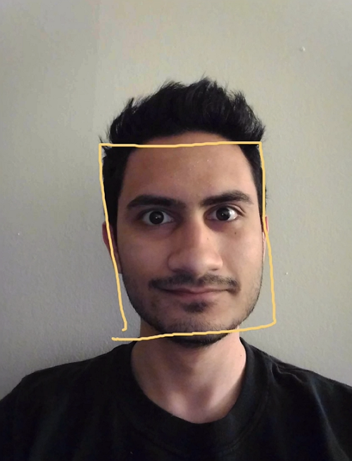
The way we’ll do it with OpenCV is by, first, using machine learning training with tons of learning examples which include positives (images that do contain faces in it) and negatives (images without faces).
Secondly, we need to analyze the features gathered during the previous step where the positives will contain face features and the negatives will contain other kinds of features.
As the features are too many, the third step is to smartly define a smaller set of features for the machine learning model to perform well. The model should be able to say whether an image has a face and where its location in the image. The technique we’re going to use for that is called Adaboost, to help us reduce the number of total features. However, even with Adaboost, that reduction may still not be enough.
The fourth step we’re going to follow is the Cascade of Classifiers which will drastically help us speed up our face detection. Now, we can send our model to the OpenCV and it’ll return to us the faces and their respective locations as we wanted.
This is our quick overview. We’re going to get into more details of all this in the next lessons.
Part 2
Before going deeper into face detection, let us see the concept of features first.
Features are quantifiable properties shared by examples/pictures used primarily in machine learning. In other words, they represent important properties of our data. For instance, we have a set of features such as color, sound, size, etc., that we can use to train an AI for bird detection. Given a new image of a bird, extracting these features will help our algorithm tell us the category of the bird.
For face detection, the computer will deal specifically with Haar features. A computer interprets the pixels values themselves, so here we have features that are close to the pixel level. We can see some examples in the image below:
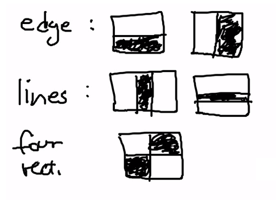
We have the edge patterns which are half white and half black (both for horizontal and vertical directions), lines, and a four rectangle pattern. The computer detects these type of patterns present in the images. But how do we extract the features?
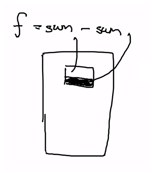
We overlay each Haar feature against our image (you can think of it as a sliding window) while computing the sum of the pixels in the white region minus the sum of the pixels in the black region. That gives us a single value f, which is our feature for that particular part of the image. Repeating the process all over our image, we end up with a ton of these features:
It may result in about 150.000 features at least (even for a small image). It is too time-consuming to get through all that info. That’s why we have the Adaptive Boosting (AdaBoost) step in face detection. It aims to select the best features to represent the face we’re trying to detect. We’re going to enter into more details of how it works in the next lesson.
Part 3
This is an introductory lesson about face recognition and its related topics.
While face detection is concerned with whether there is a face in a given image or not, face recognition tries to answer to whom that face belongs. In fact, face detection is the first step in facial recognition.
For face recognition, we do not use pre-built models as we did for face detection.
In order to build an AI, we need lots of labeled training examples, each containing an image (with the actual face) and label (the name of the person whose face is in the image) tuple. We need to go through two distinct phases with our samples: training and testing.
For the training phase, we first run face detection for all our training examples, where each will give us back one face. Then the second step is to capture the features of the faces in the images, and the third step is to store these features for future comparisons.
Now, for testing, we will have new images. The first step is also face detection, and the images here can have several faces in them. Secondly, we’re going to capture the features of all faces just like in the previous phase (notice that we have to make sure that we are using the same algorithm as in the training). The third step is to compare the captured features in the previous step to training features. Then, the fourth step is to do the prediction by having the recently detected faces associated with their closest match from the stored images under the same label. There’s also the concept of Confidence Value, which basically measures how confident is our AI in each face recognition.
Regarding the choice of the features and how to capture them, it is important to notice that it is all about using good features. You do not need a complicated or a cutting-edge machine learning algorithm of any kind if you have good features, so you should not try to compensate bad features with your algorithm.
Part 4
In this lesson, we start to work with our face recognition data set.
First, we need to set up the environment we’re going to use:

Remember to download the course files (NOT INCLUDED IN FREE WEBCLASS) and unzip the contents (included is some code for the data set loading to be quicker, and our entire data set called YaleFaces):
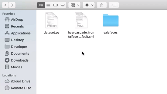
The “haarcascade_frontalface” file has code that we need only load using the CascadeClassifier class in OpenCV. The other file contains our training and testing data. Folder “yalefaces” has a lot of files varying from “subject01” to “subject15” as seen below:

Each of the subjects has several suffixes, for instance, “.centerlight” or “.glasses”, “.noglasses”, “.sleepy”, and so on. These are attributes of the same person. We want to be able to detect a person under varied conditions, that is considering light variations, or whether the person is wearing glasses or not, if their eyes are closed, etc. By taking multiple pictures of the same person with different facial expressions and poses, we tend to get better results with facial recognition.
If we open the files with an image viewer, we’re actually able to take a look at the pictures:
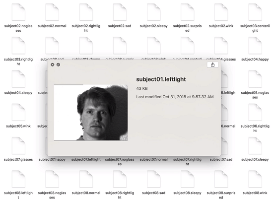
In case of trouble opening the files, you can add an extension such as “.png” to the end of each file’s name just to be able to visualize them.
As we can imagine, what happens is that all features of the same subject map to the same label (the respective person’s name).
We can even add ourselves to the data set provided we take selfies with the needed facial/environmental features (11 features, in this case), get rid of the “.pgn” or similar extension, and rename our files accordingly to the pattern of the ones in the folder. Thus, we’d be “subject16” and our selfie smiling would be entitled “subject16.happy”, for example.
We’re going to use part of these images for training, and the remaining will be used in the test phase. We’ll feed our program with all but the last picture of each subject for training, where the last picture is the one we reserve for testing.
Remember that the more pictures we have in distinct conditions the better for our face recognition outcomes. Also, our recognizer will always return us the label of the closest match it finds.
Part 5
This lesson demystifies the concept of dimensionality reduction.
The goal of dimensionality reduction is simply to receive higher dimension data and represent it well in a lower dimension. We’re going to take a Cartesian coordinate plane as an example, and we are going to reduce it from 2D to 1D.
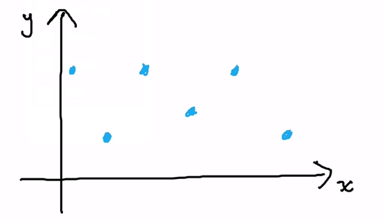
In the image above we see coordinates “x” and “y” for a group of points in a way that each point is uniquely represented in a 2D plane. But now we need to find a good axis to identify all these points just as uniquely in 1D. For that, we’ll be using projections.
Consider the “x” axis as a wall and the points as objects dispersed in a room. If we shoot various rays of light from flashlights into this room in a way that the light comes in perpendicularly to “x”, then we’re going to have the shadows of our objects projected on the wall like demonstrated below:
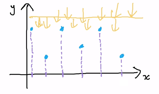
The shadows are basically each point’s coordinate in “x”. Now, similarly, if we shoot light from the side and consider the “y” axis as our wall, we have:
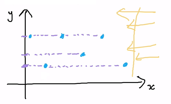
We notice that several points happened to map to the same shadow and we do not want that for our reduction. All points must be reduced to a new unique correspondent piece of information in the lower dimension. Thus, we can conclude that the “x” axis is a pretty good axis for our reduction, given that the “y” axis does not satisfy our mapping requirement. In the end, the class of algorithms for dimensionality reduction is most concerned about picking a good axis.
How do we do it for images?
We can think of an image in terms of its pixels:
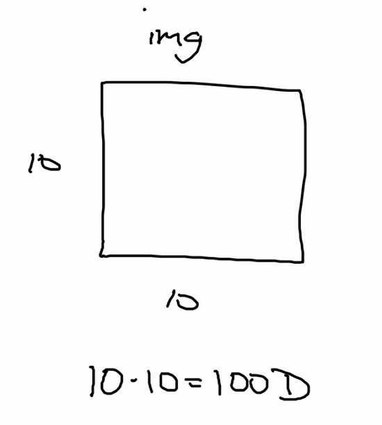
However, do we really need a hundred dimensions to tell us if two images are the same? No, we can highlight some points and reduce the whole thing to a lower dimension. In fact, actual images will be much larger than a hundred dimensions, but the point here is that we can operate more efficiently over lower dimensions obtaining the same result.
In the next lesson, we’ll see two algorithms to help us decide how to pick a good axis for our reductions.
Transcript 1
Hello everybody, my name is Mohit Deshpande. In this video, I want to introduce you guys to this notion of face detection. And I just want to give you an overview of the two different topics that we’ll be covering in the next few videos.
Probably a good place to start would be to discuss what face detection is and what it isn’t also. Face detection answers a question, face detection answers the question is there a face, is there a face in this image. This is the question that, after we’re done with face detection, we hope to be able to answer given any image. What I should say, and I’ll put this in red, is that it is not recognition. Face detection and face recognition are two different things. And it turns out face detection is the first step of face recognition.
But face detection is trying to answer the question, is there a face in this image? And then when we go to face recognition, then we can answer the further question, whose face does this belong to? I just want to make that point very clear, is that face detection and face recognition are two different things. So if we were running a face detection on this image, we might get something like, hey, look here’s a face. And then regarding whose face it is we can’t really answer that with just face detection. This is where recognition would have to come in to play.
But we’ll primarily be discussing face detection. The process that OpenCV uses, the actual process was actually released in a research paper in about 2001. It was called Rapid Object Detection using a boosted cascade of simple features by Paul Viola and Michael Jones back in 2001. And this title might sound a bit scary, but don’t worry about it all. I’m going to give you an intuitive understanding of face detection rather than the rigorous one that they go through in the paper.
The way that I want to discuss face detection is to first, in this video in particular, just give you an overview of what it all entails. Don’t worry if some of the stuff I mention in the overview doesn’t quite make sense, ’cause we’re going to get into it and really define some more things in the next few videos. I just want to give you an overview of what we’re going to be looking at in the next few videos. We’re gonna go through the entire face detection stack.
What OpenCV does is it actually uses machine learning for face detection. And that makes sense because you can’t really go around taking pictures of everybody’s face and then compare it too, instead we can learn these features. The first step is part of that machine learning. That’s the largest step. With machine learning, we need lots and lots of examples. We need tons and tons of machine learning examples.
We need positives and negatives. Positives are images with faces. And negatives then are images without faces. We need to collect this dataset of images that have faces and images that don’t have faces and manually label them as being, well, here are the images with faces and here are the images without faces. And luckily OpenCV actually has all this data already collected for us, so we don’t actually have to deal with any of that.
The second thing after that is we need to look at the features of, giving a training example, we need to extract these features. And what I mean by feature, and we’re gonna go into it a bit later, it’s kind of the essence of what a face is. We need to extract that from the positive and the negatives. The positives are going to have the essence of a face, so these features. And negatives will also have features, but they won’t necessarily correspond to faces. (whispers) Actually make this a bit clearer here, I’m going to label this as Overview.
We want to extract these features from our image. And we need to look at all the portions of our image. When we do this, we’ll find that the result we get tons and tons of features, thousands, tens of thousands, hundreds of thousands of features that we get. And these features, just numerical ways, of describing the essence of a face, for example.
We need to extract these features from all the portions of the image, and we end up with so many features. If we’re trying to apply it using that many features, face detection would take forever. So we need some way to reduce the number of features that we have and reduce them smartly, because we want to reduce the number of features, but we still want our machine learning model to be able to perform well. So given a new image, the model should be able to say, well, this image does have a face in it and here is the location of the face. We don’t want to diminish our accuracy. We want our model to stay really accurate and precise, but at the same time, we want to reduce the number of features.
There’s this technique called Adaboost that we’ll be using to help reduce the number of total features that we have, (whispers) let me get rid of that, that will help reduce the total number of features from hundreds of thousands to maybe just like a few thousand, which is in two orders of magnitude, much smaller. But it turns out that even with Adaboost, that still might not be enough. We still have thousands of features that we have to check. What they propose in their paper and what we’re going to be discussing about is this cascade, this Cascade of Classifiers. That’s gonna help drastically speed up our face detection.
There’s an f-I there, okay. This is gonna help drastically speed up our face detection because then we’re not applying all thousands, 30,000 features to each part of the image. We build this cascade thing, kind of like a waterfall. That’s where that name, Cascade of Classifiers, comes from. You can think of it as a waterfall. After we’ve done all of this, then we’ll have a great machine learning model and then we can just send it through to OpenCV and say, is there a face? And OpenCV returns all the faces and the coordinates of the faces.
And then we can use that for really cool things, like we can pass it on to a face recognition algorithm and that can determine which face the image, which faces these are, or who’s faces they are. Or we can do something, and pass it to something a little less complicated like some sort of face swapping algorithm that can extract one face, extract another face, and swap the faces. There are so many other different applications of face detection that we can use.
This is the foundation of face detection that I wanted to discuss. If the stuff that I talked about in the overview doesn’t make much sense, that’s okay, ’cause we’re gonna get into this really in the next few videos. This is just an overview. I’m going to discuss more about the intuition behind this instead of the raw mathematics, so that you have a better understanding. This is kind of an overview of face detection. Just to do a quick recap, face detection answers the question, is there a face in this image? And I made the point that it’s not the same as recognition which is going to be answering the question of whose face is this? And then I kind of gave an overview, I mentioned the first thing is machine learning examples.
We have to have a lot of the image examples with faces and without faces. OpenCV actually handles this for us. Now the next thing with this is features. What are features and how do we get them from our images or training examples? Third is Adaboost, which is gonna be an algorithm that we can use to reduce the number of features from hundreds of thousands to maybe just a few thousand. And then Cascade of Classifiers which is what they propose in their paper, ’cause even with a few thousand features, you can imagine, it’s gonna be still kind of slow.
And so Cascade of Classifiers helps speed this up. And that’s the fundamentals of face detection and then after that, there’s some parameters that we’re gonna be discussing as well. So that’s it for this video and in the next video we’re gonna be discussing this topic of features. We’ll be discussing that in the next video.
Transcript 2
Hello, everybody, my name is Mohit Deshpande and in this video, I wanna talk about features and feature extraction in the context of face detection, but before we actually get into that, I wanna start by defining what are features and I kinda wanna go through an analogy so that you kinda better understand intuitively what they are and then we’ll transition on to how face detection is specific use of these features.
So, what is a feature? Well, features are just quantifiable. Features are, first of all, they’re quantifiable. There’s some way that we describe them either numerically or through some sort of fixed list or something like that, but they’re quantifiable properties that are shared by our examples and they’re used primarily for machine learning, in our case. That’s not to say that features are only used for machine learning, but in the context of face detection, they’re used for, whoops, that should say machine learning.
They’re used for machine learning, but they have many other things, like set features and stuff, but anyway, specifically to machine learning and we care about these features because they represent important properties about our data that we can use to make decisions like categorizing or grouping.
So, let me start with an example, and let’s suppose that we wanted to teach an AI to classify different types of birds or something like that. That’s my really bad, really bad image of a bird. So, pretend that that’s a bird, I’ll even label it, bird. I’m not really good at drawing. Suppose this is a bird, so what kind of features might we have with birds? So, there are a couple that we can come up with. There are maybe, like, color of the bird or maybe like sound that it makes, there’s, you know, size, maybe how big the bird is, and et cetera.
There are many more from these that we can use and as it turns out, using a combination of these features, if we saw some new bird and we wanted to label it, we could compare the new bird’s features here with all the features that we’ve seen before in our training examples of birds and we can kinda, reasonably guess what category or group our bird should, our new bird should belong to, and so this is kind of the intuition behind it. So, let me actually just label this, AI for birds.
So, purpose we were trying to do something like this. Here some of the example of features that we might use. And then, the thing is that the AI would be given lots of these features from birds and it’d be told, well, if you have this combination of features, then this bird is a falcon or if you have this combination of features, then this bird is a sparrow or if you have this combination of features, then this bird is a duck, or something like that, and it’s been given lots and lots of these examples so that when it encounters a new bird, it finds it, it extracts these same features of the bird.
Maybe it needs a human to actually tell it, here’s the color and the sound that it makes and then here’s the size and whatnot. Maybe it needs a human to actually give those features, but when it’s given, the AI’s given these features, it can categorize this new bird as being similar in one of the categories that it already knows about, and so that kind of the intuition behind what these features are. They represent, like I said, important properties about our data and we use them so that we can better make decisions.
And so, you might be saying, well, we’re dealing with all these birds, how does this work in face detection? And so, it’s a bit different, these features here are a bit different than for faces and that’s because you have to remember that for a computer, when it sees an image, it just sees the raw pixel values. We use those pixel values to maybe give us some more understanding about the image, but initially, we just get raw pixel values. And so, our features then for this, they are a bit closer to the pixel level and so, in particular for face detection, what works well are these things called Haar features.
So, H-A-A-R and let me actually draw some, and they might seem kind of low-level. What I mean by that is, for example, here are edge features and they’re basically like, if I draw a box around it, now they basically look like this here, except this portion’s colored in. And so, this portion up here is white and this portion down here is black, and this, you know, this kind of looks like a edge, right? So, here’s one portion that’s white and here’s one portion that’s black, so this seems to detect horizontal edges.
Now, as it turns out, there’s also an analogous one that detects vertical edges, so something like this. This is also a Haar feature and so we have something that detects edges, and we also have other Haar features that detect lines, and these detect both horizontal and vertical lines. So, here’s an example of a vertical line that’s being detected, and so, this kind of makes sense, right? So, here’s the white portions and if the black portion were aligned, if I were to stack these kind of on top of each other, they would make a line.
And just like with the edges, there is an analogous one for horizontal lines and then, there’s this other unique one called a four-rectangle and it kinda looks a little unusual. It’s actually set up to be like this and this is kinda where we have some alternating thing going on here where this is, these two squares are black and these are actually all the Haar features that are used for a thing like face detection.
You might look at these initially and say, well, how could these possibly be used for something like face detection? It turns out that these work really well because the detect these low-level features that are shared among faces. They detect edges and lines and other different features of faces. It’s been shown that using these features, it works well, but so, how do we actually extract these features?
So, if you remember back to convolution, this works somewhat similarly to convolution but it’s not quite, it’s not quite the same. And so, what happens is, we basically take, where like convolution, we kind of overlay this, for example. Where we overlay, if I had an image like this, we kinda overlay one of the Haar features on top of our image here, and instead of doing this convolution operation, what you actually do is, you take the sum of the pixels in the white region minus the sum of the pixels in the black region. And that, eventually, if you do that, then you get a single value and that’s one of our features, and you basically take this and you can move it around our image, like a sliding window sort of thing, and we get a ton of features.
In fact, we get a lot of features, we get a ton of features. We can get anywhere from like, you know, maybe like 150,000 features, for even just a relatively small image. Somewhere around there, for example. Let me put an example here, ’cause it might not exactly turn out to be this, but important is, you get a ton of features and that’s a lot of numbers to work with.
So, imagine trying to get a new face and then also getting all these, trying to apply the features that we’ve seen before across all of our training examples and applying all of these to the new input image. That’s just way too time-consuming, there’s no way that you’d set this up for doing face detection, you have to come back, you know, a day or so afterwards for you to get an actual result back, but this is just way too many features and it’s gonna be way too time-consuming.
And so, this is kind of a problem that we’re encountering with this, there’s just too many features. So, what they suggest in the paper and what we’re gonna be going into more intuitively is they suggest an algorithm called AdaBoost, which is short for Adaptive Boosting, where they use this algorithm to try to select the best features that represent the face that we’re looking for. And so, using AdaBoost, we can kind of reduce this number of, you know, hundreds of thousands down to like, maybe just a few thousand of the best features. And so, that’s what we are going to be discussing more in the next video, but I just wanted to stop here and we’ll do a recap.
So, what I discuss in this video, we discussed what features are. Now, in particular, I mentioned that there’s some quantifiable properties that are shared by different examples and in our case, we’re using them for machine learning specifically. And so, I made this analogy of, if we’re building an AI to classify different kinds of birds. Some of the example features would be like, color of the bird, sound the bird makes, the size of the bird, and so on.
So, these are the kind of features and then if I give my AI lots of examples with these features and say, well, a bird with this particular arrangement of features, these values, then we can classify this as a blue jay, or et cetera. And so, we can do something similar with face detection, except we have to use low-level pixel features and that’s what these edges, lines, and this four-rectangle feature kind of is. These are like the lower-level Haar-like features. It’s been shown that using these features works really well for things like face detection.
And so, how do we actually extract these features? Well, it’s kinda similar to convolution where we take this, treat it as a sliding window, and you kinda slide it over the image, but it’s not quite convolution because we take the sum of all the pixels in the white area, subtract that from the sum of all the pixels in the black area, and then we get that single value to our feature. When we slide this over our entire image and do all that kind of good stuff, then we can end up with hundreds of thousands of features and that’s way too many.
And so, in the next video, we’re gonna talk about, intuitively, we’re gonna discuss an algorithm called AdaBoost and AdaBoost will let us reduce this list from hundreds of thousands of features to maybe just a few thousand features, but those few thousand features are actually gonna be the best of the hundred, in this case, 150,000 features. It’s gonna be the best of those, so we’re gonna discuss AdaBoost in the next video.
Transcript 3
Hello everybody. My name is Mohit Deshpande. In this video I want to introduce you guys to face recognition and some of the topics I will be discussing over these next few videos. Face recognition is the step above face detection.
After detecting a face in an image, the next natural question to ask is to whom does this face belong to? This is a question that face detection tries to answer. With face detection we’re trying to answer the question of whose face is in this image? That’s a question that we are gonna be answering with face recognition. This is different than face detection because with face detection, we’re just concerned with is there a face in this image or not? Face recognition is more specific. And you’ll see that face detection is the first step in face recognition but face recognition is a more specific question that we’re asking than whose face is in this image?
And so to answer this question, we can’t just hard code all of the values that we want in there. In fact we have to use machine learning and artificial intelligence and we have to construct an AI that, given lots of labeled examples of people’s faces, it can take a new face and say this face, it belongs to so and so for example. So that’s what we’re gonna be doing and we, actually, have to because of the way how face recognition is so specific, we can’t do something like what we did in face detection and use the pre built model because that might change depending on whose face we want to include in our data set.
I’m gonna be talking about the data set that we’re gonna be using in a future video. So just keep that in mind. So anyway, if we want to build this AI, we need lots of labeled training examples.
What are these examples? With these training examples, we need an image and then a label. This image is the actual face and this label is the person whose face is depicted in that image. This is, really, all we need. They’re just of this form image and label. There’s two phases that we need for this and right now this is, I’m gonna this out. There’s the training phase and then there’s the testing phase. We’re gonna have to do it with both phases actually. With the training phase, we have lots of examples like these. What we need to do for the training phase is to first run face detection here. That will, actually, identify the region of this image that is the face.
We’ve already discussed face detection so I won’t talk too much about that. We just use, exactly, the same stuff that we have been using with face detection. Just run the cascade classifier on this input image and then we get the results of the face back. We do that for all of these training examples. So this is for all training examples. We do this training has to go across all the examples. So for each example we’d run face detection is the first step. The second step and, probably, the most important step is to capture features of that face. That’s, probably, the most important step there is why would you, actually, detect the face?
We have to detect features about the face. ‘Cause remember with face recognition, this is a more specific question that we’re asking rather than face detection. We just can’t use those same hard features that we were talking about because those are meant to just detect general faces. You can’t really use them to detect a specific person’s face. We have to capture some features that can help us uniquely identify different faces.
That’s where this step two comes along. Once we’ve captured features for that particular face, we have to store these features with the label. Once we’ve captured these features, then we can store them and use the labels so that when we get in new training examples and new images, we can compare them to the stuff we already have seen and just take the label of the face that’s closest to whatever the new input image is.
Speaking about getting new examples, let’s talk about testing. Testing is for new images. I’m just going to abbreviate image as img. For new images, what we have to do is, firs of all, we have to run face detection again. We will want to detect the face. If the image has multiple faces, that’s perfectly fine. We will just detect all of them. With the second step, what we have to do is capture features of all faces. ‘Cause remember in the training examples there’s, generally, just going to be one face per image. That just makes it simpler when we’re dealing with training data because we have control over our training data.
With testing data, we don’t really know how many faces can be in a particular image and, actually, it turns out it’s not gonna matter. We want to capture features of all of the faces. Then after we have those features, using the same algorithm, then we can, actually, compare to training data or to training features I should say. The last step, down here is, the coolest step and that’s the prediction.
Once we have the features of all the faces in our testing image then we can compare those features with faces that we’ve previously seen, from the training phase and we can find the closest image. Once we have that closest image, then we can just take the same label that’s from the closest image and say well then this is what the person that’s depicted in this image. That’s the person that’s depicted for that face. That’s something that we can do in OpenCV fairly simply. Along with the prediction, we also get something called a Confidence Value. Intuitively that’s how confident is our AI? Is it unsure about this or is it really confident that this face belongs to this person? Anyway, this is just that OpenCV can just give us when we train our machine learning model or AI.
You can just go to new input image and you call function on it with the new input image and it will return you the label and the confidence. So that’s not something that we have to worry about too much. But the key step that I want to be focusing on is this step right here. That is capture features of all faces. Capturing these facial features.
‘Cause like I mentioned before, face recognition is more specific than detection so we have to be smart about which features we capture and how we capture the features of the face. Because if you are going into any kind of data mining or data science or anything like that, you’re gonna learn, very quickly, that it’s all about using good features. Usually if you have good features and a relatively simple machine learning algorithm or something like that, then you’re, generally, going to do better than if you have truly bad features and you try to compensate by using some really complicated, over the top algorithm. This capturing analysis of the features is, probably, the most important step in face recognition.
And so in the next few videos we’re gonna be discussing a couple of different ways that we can do that and the majority of the ways that we do this are centered around this topic called dementiality reduction. And it sounds much scarier than it actually is. I’m gonna give you a more intuitive understanding of dementiality reduction in the next video actually. But I’m just gonna stop right here and do a quick recap.
With face recognition, we want to answer the question whose face is in this image? That’s more specific than face detection because face detection is just is there a face in this image? To answer this question, we can’t just hard code all of the values in there. We have to use some kind of artificial intelligence and machine learning to identify the features of a particular face given lots of training examples, and then given a new image, we compare it with those previous examples that we’ve seen before and then you can make a prediction.
And so what I mean by examples, unless I show it here, examples are just a tubal containing the image of the face and then the label. And the label, in this case, is the name of the person. So given lots of these, we can go through the training phase and apply face detection to identify the face more specifically and then capture features of that particular face and then store those features with the labeling or the person name.
In this giant data model that has the name of the person and then the face. Multiple examples. So you can have the same person but multiple faces and we’re gonna see that that is gonna happen with the new data set that we’ll be using. It might be a person that’s smiling, frowning, the same person is winking, the same person is, you know, you just collect different images, different facial expressions from the same person.
We’re gonna get in to the data set a bit later. So anyway, that’s the training phase. With the testing phase, when you get a new image, the first two steps are the same. You run face detection and get the features. You have to make sure you get the features using the same algorithm as when you trained. And then once you have those features, then you can compare with all of the examples that you’ve seen before and then make your prediction.
That’s face recognition in a nut shell. The most important step of this is to capture these features. How do we get these features given a sub section of an image that contains a face? That’s the most important portion and that’s a portion that we’re gonna be also focusing on. A lot of the techniques that deal with that actually discuss dementiality reduction. It will give you an intuitive understanding of dementiality reduction in the next video.
This is just an overview of face recognition. In the next video, to introduce two of the algorithms that we’re gonna use for capturing these features. I’m going to discuss dementiality reduction in the next video.
Transcript 4
Hello everybody, my name is Mohit Deshpande and in this video I want to introduce you guys to the dataset that we’ll be using for face recognition.
In the provided code I’ve actually bundled this dataset in it as well. It’s actually a pretty popular face recognition dataset. It’s called the Yale face dataset and so here what some of the pictures look like over here and so when you open it up you might notice that on Linux it’ll render but if you are opening up, if you’re looking at the dataset on a different operating system, sometimes it doesn’t quite render the images of the faces because there’s no file extension, really. They all follow the same naming convention for the file name.
So, a subject and then their number and then dot and then some property about, some sort of description about the person in the image. It ends right there, there’s no .png or something like that so it just ends right there. So sometimes, I’ve had this issue on MacOS, sometimes these images don’t really render so you have to open them up in preview. In Windows you might have to actually open them in the photo viewer or something to look at them. But on Linux, luckily for us, it recognizes them as being images. Like I said, in this video I just want to get you guys acquainted to this dataset that we’ll be using and also show you how we can add ourselves to this dataset actually.
If I scroll all the way down, see I’ve added myself to this dataset as subject16 afterwards So, I’m gonna explain how we can do that as well. So, first of all, this Yale dataset, let’s pretend that I’m not in this dataset. The official Yale face dataset has 15 subjects and it’s about 11 images, or it’s exactly 11 I should say, exactly 11 images per subject. So, that comes out to us with 165 different images and so each subject has, 15 subjects and each subject has 11 images, and I should mention that these are actually gif images.
When you’re using your, if you’re trying to use your images they don’t have to be in a particular file format, by the way. You can just use them as whatever but I guess when they were making this dataset they used that particular format so what kind of image file it is doesn’t really matter if you’re going to be putting your own stuff in there anyway. Lemme, just gonna talk a little bit about the way that this dataset is set up.
So, like I said there’s 15 subjects and then each subject has 11 images and these 11 images are all different and that’s something that you should be, if you’re gonna put your own stuff in there they should be different images. You don’t just wanna use the same image 11 times. That’s not really that robust, but lets select your subject one, after the dot it tells you what conditions are in the image like, centerlight is, you know, center light. There’s one with glasses, there’s happy like a smiling expression, there’s leftlight so the light is kind of, one side of the face is a bit darker than the other. There’s one with no glasses to kinda contrast glasses. There’s a normal one which is just added in there, there’s rightlight where the right side of the face is lighter than the left side, there’s sad where they’re frowning, there’s sleepy where your eyes are closed, there’s surprised, and then I think wink is the last one. Yeah, wink is the last one.
So, you can see that for each subject they asked them to do the same thing. So like, smile, left light, center light, wink, sad, you know, and all that stuff, so those 11 images. And they’re all different. So for no glasses and normal, for example, they look really similar but they’re two distinct images and so that’s something that, when you’re creating your own dataset that’s also something that you should do. And so this is quite commonly known as the training set.
And it’s called training set because these images are what we’re gonna be feeding to our AI and telling our AI, hey this is a picture of subject one. We’ll say, here is another picture of subject one. And then we just kinda keep adding pictures of subject one and then eventually we’ll go to subject two and we’ll be like, oh these are pictures of subject two. And you give it the 11 images and it can help classify correctly and recognize whose face this is.
And one thing I should mention is that the way that I described it is, we are just gonna be ignoring what’s after the dot. We just care about the 11 images classifying the subject. They’re supposed to be different images because the more different, the more variety is in your image, or is in your training set for a particular person, the better that it’s probably gonna recognize your face. Because if you take one picture and copy it 11 times and try to teach the classifier that, it’s just gonna pick up the same features 11 times.
So that’s not really that useful. Which is why there’s all these different conditions like center light, there’s one with glasses or without glasses. If you don’t actually wear glasses then you can just borrow your friend’s or do something else with that. When you’re doing your dataset they don’t have to match up with this. You can just take 11 images from different angles and different facial expressions.
And one thing I should mention, is that you might be tempted, looking at this, to see if you can do sentiment analysis and that’s a whole ‘nother field in computer vision. What I mean by that is, given a picture of a face, can you tell if it’s smiling or winking or stuff like that. You might be tempted to think that you can do that given this image set and you might be able to but I don’t think it’ll work that well. In fact, there are actually a lot of APIs that are starting to come about that actually already do sentiment analysis.
So, you can usually just piggyback off of one of those. If you were trying to do sentiment analysis what you would do, your training set will then be different. You would need, just for one subject, you would need multiple pictures of them, like, winking, or multiple pictures of them being happy, or multiple pictures of them sad, and you know, so on and so on. It’s really all dependent on the training set and so I think that’s pretty much covers all that I wanted to cover about the Yale face dataset and so in the next few videos, actually in the next video I’m gonna show you how you can put yourself in this dataset and some of the stuff that has to go with that.
But, I guess I’m gonna stop this video right here for this kinda introduction to the dataset here. Okay so, I’m just gonna do a quick recap, so, for our face recognition dataset we’ll be using the Yale face dataset and there are plenty of other datasets out there. I think AT&T has a face dataset, but it’s way bigger than this so I just wanted to, I chose this dataset particularly because it’s not a massive dataset, it’s like 165 images so you can skim through them really quickly but some of the other datasets have hundreds and hundreds of images so it just gets kinda tedious. Plus, when I actually get to the training phase that might take a bit longer for more images of course.
But anyway, this is the Yale face dataset and it’s split up so that there are 15 subjects and each subject is uniquely identified by a number and each subject takes 11 images. And these images are unique images in the sense that they’re not just the same image copied 11 times. So, here’s all these different kinds of images of different facial expressions and different lighting conditions so that we can really try to make our AI more robust in these changes. So it’s 15 subjects, 11 images per subject and we’re gonna be using this dataset for training our AI.
I guess I wanna stop right here with the Yale face dataset and then in the next video, if I scroll all the way to the bottom here, you can see I managed to put myself into this dataset and so if you wanna add your own face recognition here then you have to add your own face in here and there are some nuances that you have to kinda look at when discussing that so this is probably where I’m gonna stop right here. In the next video I’m gonna show you how you can add yourself to this face dataset.
Transcript 5
Hello everybody, my name is Mohit Deshpande and in this video I want to introduce you guys to this notion of dimensionality reduction and so name sounds much scarier than it actually is so let me just kinda give you an intuitive understanding of what it is and then we’re just gonna look at an example of how we would do this and the reason we’re talking about this is because two of the algorithms that we’re gonna be discussing, particular eigenfaces and fisherfaces are used for face recognition.
Under the hood they actually use two algorithms called principle components analysis and linear discriminant analysis and both of these are a kind of dimensionality reduction and so this video is gonna kinda introduce you to this concept of dimensionality reduction so that we can talk about the two face recognition algorithms that you use here. So what is dimensionality reduction?
So this just describes a set of algorithms whose purpose is to take data in a higher dimension so higher dimension data and represent it well in a lower dimension data, in a lower dimension basically and so I’ve been using this word dimension a lot so here’s an example actually that I’ve drawn of a scatterplot, this is just a plain old scatterplot, nothing fancy about it so this scatterplot is actually in 2D and in the example that we’re gonna be using, we’re primarily gonna be going from two dimensions to one dimension and so 2D is a plane and so this, no, is our x, y plane.
This is also called the Cartesian coordinate plane but the point is it’s in two dimensions and why it’s in two dimensions is because we to represent any point in this coordinate system, you need two things to identify uniquely.
You need an x coordinate and a y coordinate so each of these needs an x coordinate and a y coordinate to uniquely identify this and so you know kind of the examples that we’re gonna be going from is 2D to 1D and so what is one dimension, well that’s just a line, it’s a number line right so we only need one thing to uniquely identify a point on a number line, you just a need a single, a one component basically so that’s what I mean and so then this is kind of what we’ll be using for examples because and this can be applied to, like going from three dimensions to two dimensions but it’s just easier to draw it if it’s from two dimensions to one dimension so I’ll just gonna be using this for now.
So yes, so what we’re gonna be doing is we need to find a way to take this data in two dimensions and represent it well in one dimension and so you might be asking well wait a minute, how do we do that if the data’s in two dimensions, you know how do we just cut off one portion of the dimension, you know.
So what we’ll be doing is we’ll be doing these things called projections and to handle this intuitively, let me explain to you what a projection really does so how we can reduce dimensionality is commonly through finding an axis to project our points down to a lower dimensional axis to project our points down to so what I mean by, I’ve been using the word projection but what I mean by that is that suppose that we wanted to project all these points onto the x axis, so what I mean by that is we want to take all these points and then plot them along just the x axis and because the x axis is a line, then we’ve effectively done our job.
We’ve taken something in 2D, the scatterplot, in two dimensions and we can represent that in one dimensional line. So to do this, we have to use projections so what a projection is is imagine I have like imagine I have like a flashlight or a series of different flashlights and this x axis was a wall and these points on the scatterplot were like some sort of object that’s kinda in the way and so what I do is I take this light and I make it so that it is perpendicular to the x axis.
In other words if one’s a right angle so I shoot rays of light, I have my flashlight and I keep you know shooting these rays of light onto this so that they all kinda go down in this way and so what happens is these points are in the way so these points are actually gonna cast shadows along this wall right so these objects are gonna cast shadows and so where along the wall are these objects gonna cast shadows?
Well if I have a ray of light coming in here, then it’s gonna cast a shadow and it’s gonna be right here is where it will, where the shadow will be on the wall and so I can do the same from this point, I can, you know if I have a ray of light going right here then it seems that this point right here would also you know, have a shadow right here. Let’s do this for all the points so let me just go back to this point and if I draw this point and I draw this line from the shadow, it’s gonna appear roughly right here and so if I do this point, then the shadow should appear right here ’cause if I have my rays of light are gonna be casting, you know these objects are gonna cast shadows and I keep doing this and you know I will have an object right here now and then I have this right here.
Okay and so now what I’ve done is I’ve actually taken my points and projected them along the x axis so I’ve done my job of dimensionality reduction. Now I have points that are in one dimension. Right so these points are along a line and so what we’ve done is using projections we’ve taken data in two dimensions and projected it into data that’s in one dimension and this representation, this particular one is actually a pretty good, we’ve chosen a pretty good axis actually to begin with.
The x axis so I want to show you what it’d look like to choose a good axis first and then we’re actually gonna go ahead and choose a bad, let’s choose a bad axis to project onto now so the x axis, this is you know how we did projections so now let me actually project along the y axis and so you know how do we do something like how do we project along the y axis, well we just take our light and we make it so that it’s now gonna be going to the left so now I can take my flashlights or something and then now I’m gonna make them go to the left and so now let’s do the same thing with projections.
Well then if I take this point here, it’s gonna be right here where the light is gonna cast a shadow so that on this wall of my y axis if I have some light here, it’s gonna cast a shadow like this. When I pick this point, then I get something like this here and so if I get this point though, you can see that it’s actually kind of overlapping with point and so these two points are kinda like the shadows will be the same shadow like right here and the same for these three points actually.
It turns out that these three points actually share, if I, you know, put two points, if I put these objects in a line and I cast some light under the shadows, they’re gonna kinda like overlap here and so we just get one point here and so you may be thinking well hey great, this is good because we’re kind of reducing our, we’re reducing the number of data that we have but it turns out that this is actually isn’t a good, an axis to use. It’s not a good line to use.
The x axis was good and so the class of algorithms for dimensionality reduction are most concerned about picking, picking a good axis so that’s kinda what this whole notion of dimensionality reduction like the two algorithms that we’re gonna be talking about in the next video, they’re most concerned about picking a good axis to cast our light, to cast our shadows on and this is what’s called a, what’s known as a projection and so you know, how does this, I’ve been talking a lot about these like scatterplots but how does this work with images actually because the two algorithms that we’re gonna be discussing are dealing with images.
Well it turns out you can think of the dimensionality of you know, an image so like suppose I have this, is a 10 by 10 image here so you know what is the dimensionality of this image? Well the dimensionality is equal to the number of pixels in this image so this image is actually in a 100, it’s a point in 100 dimensional space and that’s really hard to think about, I mean most experienced mathematicians have difficulty imagining, visualizing the fourth dimension and I’m asking you to think of something in 100 dimensions.
That’s just not, you know that’s not good and we kinda get the same thing, we kinda get the same principle when we were discussing face detection is do we really need a hundred dimensions to tell us if two images are you know the same or not of if two faces are identical and it turns out that no, we really don’t and so what we’re trying to do is take something in like 100 dimensional space and bring it down to something like, I don’t know maybe like 10 dimensional space or something like that and then we can just compare the two, the input image, we do the same thing with the input image is we convert it to 100, we convert it from 100 dimensional space down to 10 dimensional space or something and compare the two.
You intend to natural spaces very impossible to visualize while what it might be that 10 things that can identify a point in 10 dimensions will you know work. Maybe 10 numbers works well and we can kinda reduce, you know our dimensionality of the image and all this is gonna be kind of happening under the hood by OpenCV so you don’t have to try to wrap your head around a hundred dimensional space. But the principle here is the same.
We just wanna take something that’s in a higher dimension and move it to a lower dimension with a simple representation so that we don’t have to deal with like a hundred numbers representing a face where in this case versus 10 numbers representing a face and in reality the images, the input images are gonna be much higher than a hundred dimensions. This is actually really small but we want to reduce the dimensionality so that we can compare two images in a relatively, lower dimensionality and so we can get a good result that helps improve accuracy and efficiency and so that is just and actually just a quick cyber.
As it turns out, you can use the same dimensionality reduction techniques to take a point, take an image and actually plot it on like a scatterplot and you know if two images are close to each other, that would mean that these two images are actually similar like they’re really close to each other and so you can do all sorts of cool things with dimensionality reduction but it turns out it’s also super useful for face recognition and so there are two algorithms that we’re gonna be talking about in the next few videos about how you know and they describe basically ways that how we can choose a good access so anyway, this one messed up right here and
I’m gonna do a quick recap so with dimensionality reduction, what we’re trying to do is take something that’s in a higher dimensionality and represent it simply in a lower dimensionality so I showed this example with the scatterplot.
I want to take this two dimensional data in x and y and just represent it on a line and so a way to do that is we use the thing called projections and so projections, imagine the axis that you want to project on is a wall and you have a light, like a flashlight that’s projecting in this, like projecting light rays in perpendicular to this wall so that the points are like random objects and so when you cast the light that will make shadows along the wall and you plot where the shadows are on the wall and then that gives you, you know, you can now successfully take data from two dimensions and put it in one dimension by looking at the shadows that these cast.
It’s also kind of why they’re called projections ’cause you would think of it as a light projecting a shadow basically so that is dimensionality reduction and then the next two videos, we’re gonna be discussing two particular algorithms that we can use to answer those question of how do we pick a good axis so I’m gonna get to the first one called eigenfaces and principle components analysis in the next video.
Interested in continuing? Check out the full Build Lorenzo – A Face Swapping AI course and Build Jamie – A Facial Recognition AI course, which are both part of our Python Computer Vision Mini-Degree.
