You can access the full course here: Video and Optical Flow – Create a Smart Speed Camera
Table of contents
Part 1
In this lesson, you will learn the basics of videos, and how function notation can be applied to find pixel intensities of videos.
Videos are a sequence of images (called frames), which allows image processing to handle videos.
The rate at which the images change is called the frames per second, and is known as the FPS of the video. A common example of this is 60 FPS, which means the video shows 60 frames every second.
For images, a function I can be applied to the image so that I (x,y) = p, where x and y are coordinates, and p is the pixel intensity.
For videos, there needs to be additional information to find the pixel intensity, as there are numerous frames to choose from. The parameter t needs to be added, with t being when in the video the desired frame is located. Then, adding t to the image function, I (x,y,t) = p for videos.
Part 2
In this lesson, you will learn about the basics of optical flow and the mathematics of it.
For images, the only information that you can access is the spatial positioning in relation to other pixels. The benefit of videos over static images is that it adds temporal information, so that you can know not only the location spatially, but also when it exists. This is what allows optical flow to function.
Optical flow is type of computer vision technique that is used to track the apparent motion of objects in a video. Optical flow can be used to track objects, stabilize and compress videos, and allow AI to generate descriptions of videos.
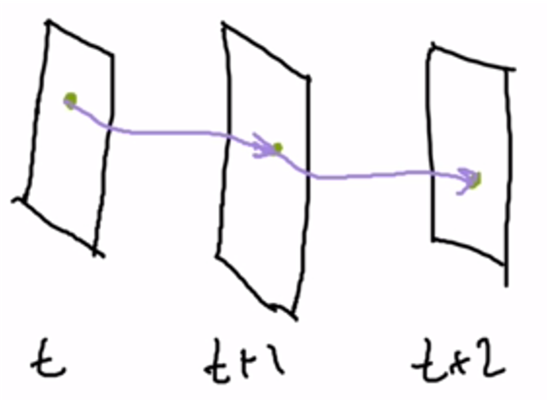
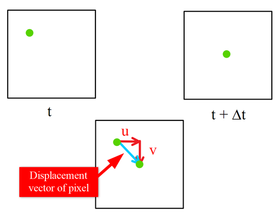
Optical flow functions by tracking a pixel through consecutive frames. This allows for the path of that pixel’s movement to be generated, as shown in this image.
Optical flow makes two assumptions that drastically simplify this process. These are:
- Pixel intensities don’t rapidly change between consecutive frames.
- Groups of pixels move together.
These two assumptions apply when a video is smooth, as pixels should change gradually and not teleport around the image. These assumptions apply for almost all real world videos, but can be broken if someone specifically edits a video to make that occur.
When analyzing videos, the pixel you are tracking will be displaced from its original position by some value u in the x direction and some value v in the y direction, as shown in the image below. The goal of optical flow is to find the u and v values, as they allow you to create a displacement vector and track the pixel’s path.
Part 3
In this lesson, you will continue to learn about optical flow, with this lesson providing more information about the mathematics behind this technique.
To recap from the previous lesson, the point of optical flow is to find the displacement vector of a pixel, with u representing the change in the x direction and v representing the change in the y direction. In the image, t represents the time at which the frame occurs, with Δt representing how much time has passed since the previous frame.

Using the function notation from the earlier lessons, the pixel intensity for the frame at time t can be stated as I(x,y,t). The pixel intensity for the second frame can be stated as I(x+u, y+v, t+Δt).
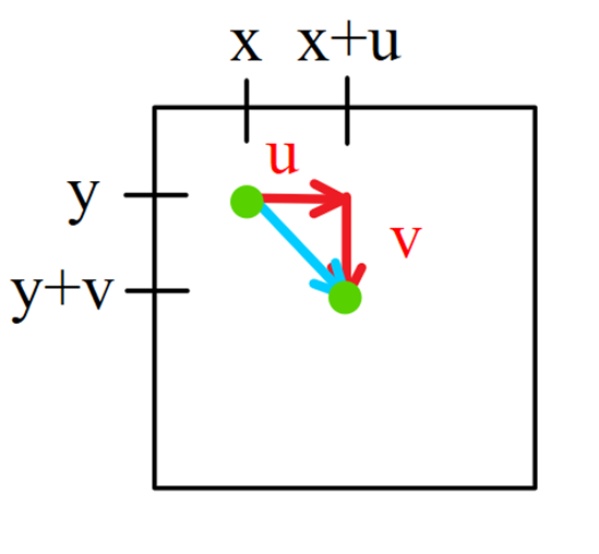
These two functions should be equal, due to the first assumption of optical flow, meaning that I(x,y,t) = I(x+u, y+v, t+Δt).
After using some calculus, this equality turns in to the equation Ixu + Iyv + It = 0. Ix represents how much the frame changes horizontally, Iy represents how much the frame changes vertically, and It represents the difference in time between the frames.
Ix, Iy, and It can all be computed, so the equation comes down to solving for u and v. There are numerous methods to solve this, but as they require calculus and linear algebra, this course will not be covering all of them. Certain techniques which will allow you to find u and v will be addressed in later lessons.
Transcript 1
Hello everybody, my name is Mohit Deshpande, and in this course we’ll be building an app that can track objects through video and actually determine what their speed is based on certain properties of our camera.
So we’ll be able to build this. And I’ve shown this visualization here. You can see that I have a pencil here that I’m waving, and the points are being tracked on that pencil, and we can get the speed readings from those points. And so that’s what we’re gonna be building in this course. And you can try this out with other objects as well.
So kind of the big topic that we’re gonna be discussing is called optical flow. And optical flow allows us to take points in video and track them through each frame. So we’re gonna discuss how that kind of works. And we’re also gonna talk a little bit about camera intrinsics, because we have to know a little bit more about our own cameras before we can get accurate speed measurements. And lastly, I’m gonna show you how we can visualize these optical flow patterns.
What I mean by that, and you saw it in the previous slide, how I can kind of draw on top of my frames and we can kind of draw a path. So we’ve been making video courses since 2012, and we’re super excited to have you on board. Online courses are a great way to learn new skills, and I take a lot of these courses myself.
So general courses consist mainly of video lessons, and you can watch, re-watch them as many times as you want, and at your own pace. Everything we do in source code is downloadable by the way. And when I’m coding this stuff in the videos, I really, really recommend that you code along with me, because coding along helps you learn material better than just watching code. The last thing that I wanna mention is that students who get the most out of these online courses are the same students that make a weekly plan or schedule and stick with it based on your own availability and whatever your learning style is. And remember that these videos, you can watch or re-watch them as many times as you want, so that kind of gives you a lot of flexibility.
So at ZENVA, we’ve taught programming and game development to over 200,000 students, over 50 plus courses since 2012. And a lot of these students have used the skills that they’ve learned in these courses to advance their own careers. Some have started companies and published their own games and apps. So thanks for joining, and I look forward to seeing the cool stuff you’ll be building. But now, without further ado, let’s get started.
Transcript 2
Hello, everybody. My name is Mohit Deshpande. And in this video, I want to first discuss what videos are, and we’re going to have kind of a change in notation before we get into optical flow because it just becomes easier to work with and understand optical flow if we have this change of notation kind of thing.
So before we can talk about it though, we have to formally define videos, and that’s because optical flow actually operates on videos. So we need to have a good understanding of what is a video before we can really get into optical flow. So we know that we can represent images as matrices for grayscale, but what about video?
So what is videos? So to kind of answer that question, think about some of the videos that you’ve seen at the movies, or on your TV, or your computer, tablet, phone, YouTube, and what not. So it seems that when you watch a video on YouTube or something, you can pause it and you get a still image, right? And so what does that kind of imply about videos? Well, you can take a scrubber or hit the rewind or forward button and kind of go through each of the still frames. So that produces something enlightening about video and that is that video, video is just a sequence of images.
Sequence of images. Because, you know, you can pause a video and kind of scrub back and forth using some sort of scrubber or a fast-forward, rewind sort of thing. And so you’ll notice that videos are just a sequence of images and they’re played fast enough that they don’t look like still images. They look like one fluid motion into what we call a video. And this also becomes apparent if you ever had like some kind of sticky notes, like a flip book, or something.
You can draw each image and when you flip through them fast enough, it looks like one continuous animation, for example, like that. So that kind of gives you the background for videos. They’re just a sequence of images. And in fact, if you’ve heard of something like FPS, right? That’s actually called frames per second. And that’s just like the speed. That tells us how many frames are being shown in one second.
In the context of videos, these still images, we actually call them frames. So we say that video is actually comprised of different frames. Rather than images, we just say frames. And so when you see something like FPS, that means frames per second. That’s how many frames are shown per second. And you know, you might have heard values for this like 60 FPS is a very common number to see next to frames per second, and that’s saying that you see 60 frames in one second. That’s 60 frames, 60 still images in one second.
So this is moving pretty fast. So the frames are moving pretty fast. You can also have lower FPS, like 30 FPS or 15 FPS. And as you decrease the FPS, it becomes clearer that you’re looking at still images played in succession rather than one continuous motion. But anyway, so that’s just kind of an intuitive understanding of videos.
But now, if we want to formally discuss videos, then we have to change the notation a bit. Particularly, we have to go from a matrix notation to function notation because if we try to stick with matrix notation when we’re discussing videos and we have to talk about these things called tensors, and that just gets like way beyond. It kind of gets out of control at that point. So let’s just start with images first. With images, let’s kind of start with images and then convert from images to video. We’ll start with this notation. So with images, we know that they’re matrices, and we can represent grayscale as matrices.
And so what we can do is, analogously, we can define a function, I’m going to call it capital I, that takes an X and a Y coordinate and returns some pixel value or intensity. And it turns out when it comes with videos, we’re only concerned with pixel intensities. So we can drop any colors and just consider a grayscale. But it turns out that this is like an analogous notation to matrices. So this is, you know, kind of the function notation, function notation, here for images. And it’s kind of like if you were trying to find a book or something in a library, whether that’s a physical library or like some online library.
You know, if we wanted to find a particular book, we need some information about it like it’s book number, the genre, the author’s name, or what not, and you know, et cetera. But when we have that information, we can find the book that we’re looking for. Each book in our library is uniquely identified by some group of attributes or values. Usually, that’s something like title, author, and book number, or something like that. So you know, given a set of values, if I tell you three values, it points to a unique book. It’s never like if I tell you three values, you have two possible books you can choose from. It’s always if I tell you some set of values then you get the unique book.
When we’re using this notation, think of our library as the image and that X, Y is the information that we need. And so this function I is kind of analogous to the act of finding a book that we want or finding a particular pixel intensity that we want. So this is saying that at, you know, this gets us at we’re basically getting the pixel value at X comma Y. And you can think of these with the old matrix notation as king of being the indices.
If we have an image, then we can just like have an image here. And then at a particular location, X comma Y in our image if we think of this as a coordinate plane, there’s some pixel intensity P that’s there. So that is the kind of notation for images. So like, you know, given an X and a Y, X and Y are unique, and so we can get the pixel value. But for videos, this is a bit different ’cause we can’t just use X and Y because we have that additional component of, well, in which frame are we doing this look up?
So, this works well for a single image, but when you have a sequence of images like videos, then we can’t just use X, Y. We need actually one other parameter and I’m going to call that T, and then this will get us a particular pixel value. And so this T represents where, when in the image, or when in the video, I should say. So this kind of represents a when in our video, which frame do we find, you know, look at the X and Y to get a particular pixel intensity.
So this is kind of like a spatial position here and this is a temporal position here, ’cause this has to do with the spatial positioning of the pixels in a particular frame. This has to do with when is that frame. And so that’s why for videos, we need three values here instead of just two images for images because just using X and Y isn’t sufficient for finding a particular pixel in the video because (mumbling) this video, we don’t have a single image, we have a sequence of images, so we need another parameter to tell us where in the duration of the video that we can be finding this pixel. But anyway.
So for video, we need three parameters. So this is kind of the notation that I’m going to be using for the rest of this course because for optical flow, it just becomes easier to deal with this I function rather than dealing with matrices, like I said, ’cause then we have to get into tensors and it just gets kind of out of control at that point. But anyway. So going forward, we’ll be using this notation to look at optical flow. So I guess I’m going to stop right here and do a quick recap.
So in this video, we discussed, well, videos, and we defined them as being just a sequence of frames. These frames are just like, you can think of them as being still images. And they’re played so fast, we see them appear so fast that they appear to be like one continuous motion. They appear to have motion. And so, you know, like, frames per second is a common measure of this and frames per second tells you how many of these frames do you see in one second. So common values for this were, like I said, were like 60. You’re seeing 60 frames in one second, so that’s pretty fast.
So I just kind of gave you an intuitive understanding of videos, then we moved onto this change of notation from matrix notation to function notation here. So I just described this I function as basically like a lookup table. So we go to the pixel at coordinate X comma Y in our image starting, you know, at the standard image coordinate system. And then P is the pixel intensity that we get at coordinate X, Y. And then for videos, I said that X, Y just isn’t sufficient, so we need another parameter, T, and then tells us when or what frame we’re looking at, basically. So when in the duration of the video do we look. So kind of moving forward, we’re going to be using this notation.
So that’s where I’m going to stop with this video, and then actually in the next video, in the next sequence of videos, I’m going to kind of give you an intuitive understanding of optical flow, and so we’ll kind of get through that. So we’re going to start optical flow in the next video.
Transcript 3
Hello everybody my name is Mohit Deshpande, and in this, just gonna start the sequence of videos that are just gonna kind of give you an intuitive and complete understanding of optical flow and we’re also gonna get a little bit into the mathematics of particularly the actual equation for optical flow and I’ll talk about some of the stuff there. I won’t be going too far into the mathematics, but I just wanna kind of give you, I want to start off by giving you more of an intuitive understanding first and then we can kind of take that intuition and solidify it into more concrete math terms.
So first of all, we have to kind of talk a little bit about what this is and the motivation behind this. So images are great. Videos are even cooler, because we have more information in a video than in an image. Because in an image we just have the spatial positioning of the pixels. That is where they are in the image relative to each other. So that’s all we get in an image but in a video, we get the same spatial information but we also add an additional temporal component. Meaning we not only have the location of a pixel spatially, but we also have when does this pixel exist? Maybe it’s only at one particular frame. Maybe it exists for a sequence of like 50 or 100 frames or something like that.
You get this kind of additional, you get this additional information about the time duration of pixels, and so optical flow is kind, so a lot of, when you have this additional information it really opens up a lot of doors as to what we can look into.
And so optical flow is one of these doors. It is a computer vision, I’ll just write this down. It is a computer vision technique that is used to track the apparent motion, apparent motion of objects in a video. So using this technique of optical flow, we can actually find a pixel value or you can kind of make this more generic like an object and we can track it through the video. And so you know later we can draw kind of like a path, we could draw like a pathing. I’m gonna show you how to draw this, just a second, but this is actually really interesting because of optical flow because first of all it’s not just used for things like object tracking through videos.
It actually has a ton of different applications that we’re gonna be discussing in a later video. Like video compression, video stabilization and actually just recently there’s been some very recent research, that is using optical flow patterns to help give descriptions of snippets of video. You can give this AI a snippet of video, and it will generate a language or generate like a video description, and that’s really cool in optical flow features, turns out that optical flow is actually pretty useful to this sort of thing, but we’re gonna discuss this stuff at a very, very top level in a later video, but let’s first derive the intuition behind optical flow. So remember that if you want to track an object through the video, remember that on a computer level we only have access to these raw pixels.
So suppose I have like a frame here, here’s one frame, and then here is another frame. We only have access to the raw pixels and I kind of drew these, these probably should be the same size, but we only have access to, here is, oops, here is a frame t, maybe here’s a frame t plus one. And then I’ll draw another one short. Maybe here’s a frame t plus two and whatnot. What we’re trying to do with flow is to take a point here and a point here, and then track it through through this frame. It’s gonna go here and then it kind of goes down here, and this is what we’re trying to do with flow.
And so to do this, we consider two consecutive frames, and we kind of build the path and just kind of, it becomes like connect the dots. You have, where the dots are the position of this particular pixel at each of the frame, so this is kind of connect the dots. Initially, at first glance this might seem impossible because you have to consider so many things like the size of the frame, how do we know which pixels are which and whatnot, but it turns out that there are two assumptions that optical flow makes that really help simplify this.
So assumptions and we’re gonna be using these assumptions in later videos. So there are two assumptions that optical flow makes. One is that pixel intensities, pixel intensities don’t rapidly change don’t rapidly change between consecutive or successive frames. So what I mean by this is that this pixel value don’t just, in two successive frames they don’t just immediately change. So that would be like, in our case at least that would be like this pixel value is green here and in the next frame, it becomes like blue or something like that. So the assumption that flow makes is that this doesn’t happen. If you consider things like, like this has real world implications.
So the frames are taken such that there is such little time between them but unless you were actually video editing each frame, you wouldn’t really encounter something like this. Now this is not to say that maybe pixels don’t change after a longer period of time. That’s fine. But this is just saying that they don’t just flip between two consecutive frames and the time between each frames is like really small. If your pixels are flipping in between frames that’s kind of weird. Maybe there’s like some video editing stuff that you can do to make that happen, but naturally this doesn’t really happen. Anyway that’s the first assumption.
The second assumption is that groups of pixels, groups of pixels move together. So what I mean by this is that the pixels don’t really move between frames. This is just like saying that pixels don’t teleport. So if I have a pixel over here like a group of pixels here, they’re not just gonna like jump to, that are at the top of the image, they’re not gonna jump to the bottom of the image in the next frame there. That kind of hinders good flow tracking when pixels just teleport. Ideally you don’t want your pixels to teleport between frames, and again this is also you want the motion to be smooth and optical flow works really well when the motion is smooth, not when it’s like jumpy or teleporting.
So like I said, these assumptions have real world implications, so in the real world if you’re taking video, stuff just doesn’t teleport everywhere. That would be really bad. These assumptions are perfectly valid to make based on the real world implications of this. Now there are ways if you were take a video and do like some video editing stuff, you could break these assumptions intentionally but we are not really going to be considering that. I’ve kind of drawn a picture here, but let me draw like a, let me draw a, just almost two frames.
And so actually I’ll probably draw a third one right here. Yeah okay so of course I have my pixel here and here’s one particular frame and I’m gonna color that green, then here is the same pixel in the next frame here, and so let me actually on the label use frames.
So this will be something like t and this will be something t plus delta t and what I mean by delta t is that just some short amount of time has elapsed. So if I were to look at both of these pixels in the same context, then I’m gonna get something like this. Where there are two different, they’re a little bit apart here and so the problem of flow, the thing that we’re trying to solve here on this red here is, I want to find there is some displacement. So the pixel moves in the x direction by some amount u and down in the y direction by some amount v.
So the challenge of flow is to find this u and v that it moves, because if we have that then we track the path. Then now that we have this displacement then we get this thing called this displacement vector, we know how much this pixel has moved. I’m gonna stop this video right here.
In the next video we’re gonna talk a little bit more about the solution to this but yeah this is the problem that optical flow is trying to solve. How we find these values, this u and v? So I’m gonna stop right here, do a quick recap, and then we’re gonna kind of continue flow in the next video. So I’ll just do a quick recap here.
We discussed optical flow and it’s the computer vision technique to track the motion of objects through videos. If here it frames a video, I want to build this path throughout my video tracking a particular pixel. So this can be really challenging but there are two assumptions that optical flow makes that are kind of rooted in the real world.
That is that pixel intensities don’t rapidly flip between frames and that pixels don’t teleport are the two assumptions and so these are valid assumptions to make in everything, but in specific I kind of showed a sequence of frames here, but in specific we get two frames that are some time unit or part of some delta t, then the problem flow is to find this u and v, like how much has this pixel moved in the x direction and how much the pixel has moved in the y direction?
So that’s the problem of flow and then in the next video, I’m gonna kind of take this intuition and make it a bit more concrete using mathematics, so we will get to that in the next video.
Transcript 4
Hello everybody, my name’s Mohit Deshpande, and in this video, we’re gonna be delving a little bit more into optical flow and add a little bit of mathematics to this.
So if you recall from the previous video, the point of flow is to find this u and v, and we have two assumptions. Actually, let me take this image and expand it out a little bit so you can see it a bit better. So I have two consecutive frames here, and then in the resulting frame, so we’ll have, let’s say we’re considering this pixel here in frame at time t, and then this same pixel is over here at the frame at some time t plus delta t, and so delta t is the elapsed time. So that’s what delta t just means, delta just means difference, and so this t plus delta t just means that from this frame a little bit of time has elapsed and now my pixel is in a different location. So let me start here, and then you know, sort of like over here-ish.
And so the point of flow, like I said, in some elapsed time, this pixel has moved to the right by some amount that I’m gonna call u, and then has moved down by some amount that I’m gonna call v. And so that’s what we’re trying to find with optical flow, and actually if I do this, I can complete the triangle. So this is what we’re trying to find, we’re trying to find this u and this v with optical flow. So how do we find this u and v? Well, we use mathematics. So I provided an intuitive picture here, but let’s actually kind of formalize this picture a little bit.
So if you remember at the first assumption, this is saying that pixel intensities don’t rapidly change between consecutive frames. So it’s reasonable to say, and I colored it in such a fashion that these two pixels at different frames have the same pixel intensity, and just to remind you, intensity is just when we drop the, we’re just gonna drop any sort of color and we’re just gonna consider our pixel intensity. So it’s reasonable to say that at these two instances in time, at some t and t plus this delta t, at this point in time, the pixels have the same value. So actually if we go back to, if we use our notation, our function notation, this is saying that the I function applied to this is equal to the I function applied to this.
So let’s actually, you know let’s write that out a bit more formally. So what is the pixel intensity in this frame? Well this pixel intensity is I(x,y,t) because this pixel, let’s say that it’s a coordinate x comma y. So now the question is, what is the pixel coordinate here in terms of x and y, and u and v? Well, this pixel, the x coordinate is the same x coordinate here plus this small change u. So this is gonna be x plus u, because here, the x coordinate is like right here, and the x coordinate here is new here, and so this difference between them I said here’s x, and then here is x plus u, because I’m moving u units to the right.
So this is x plus u, which is why I call it x plus u, and then similarly if this were y, then this is then y plus v. So in this coordinate is x plus u, y plus v. And so now I can write this frame as being I, and then the x coordinate of this pixel is x plus u, because I’m at the same, here’s the coordinate for the first frame and here’s it for the second frame, and so I’m moving right u units. So that’s x plus u, and then comma, what’s the y coordinate? It’s y, which is the same coordinate here, plus v, because remember here’s the initial coordinate in frame t, and then in t plus delta t, I’m moving down by v, and so this is y plus v. And so now what’s the time? Well, I just told you what it is, it’s t plus delta t. T plus delta t.
And so now I’ve written this frame, this next frame, in terms of this current frame, and so actually just to make this clear, so this is movement in x direction, movement in x, which is what u is, and then v is movement in y direction, in y axis, I should say. Then x axis. Right, so then these are just the displacement, and this is movement in time. Movement in time. Time axis, so just like the next frame. So that’s what these three values represent. And so I can represent these two pixels here, but what is I? I is just a measure of pixel intensity. 3
And what is I here? This is just a measure in pixel intensity as well. And so if you remember from the first assumption that pixel intensities don’t rapidly change between two successive frames, these are actually equal. And so this is the optical flow equation here.
This is a really important equation, and it’s not quite in a term that we can use quite yet. So this is an important equation. So this is saying that at some time t, the pixel intensity here, is equal to the pixel intensity at, you know some time has elapsed between one frame and the next frame, and we can write it in terms of this u and this v.
And so just you know, take a second and look at this equation and make sure that it logically follows that from our first assumption that these two things should be equal, and that the x coordinate of the pixel in this frame is the x coordinate in this frame plus u, and then y plus v, and then t plus delta t, and so like the position here so that everything, so that this makes sense. Actually, let me draw these markers as well since I drew it for the x axis. And so hopefully this makes sense.
If you have any questions, I guess I’d just hopefully post a comment, but we want to find the values of u and v but they’re in our function. So how do we separate them from our function? And it turns out that we actually use calculus to do this. So I’m just gonna put dot dot dot calculus. I’m just gonna put calculus, and I’m just gonna write down the final equation here, and that is I sub x u plus I sub y v plus I sub t equals zero. So this direct conversion from here to here actually using calculus, I’m not really gonna talk about that at all, but, so these two things I will talk about.
So we end up with a single equation here, and x, so this I sub x represents how much the frame changes with respect to the x direction horizontally. This y is how much y changes, or how much the frame changes with respect to the y direction, and so vertically, and then I sub t is just the difference between… Is the image difference between the two frames, so how much do the frames change along the time dimension. And so it turns out that we know this. I’m gonna put like a check mark. We can compute this, we can compute this. We compute this, ’cause it’s just an image difference and then these two things we can actually use convolution to compute.
So we have this equation of variables, and it turns out that these things, we can compute. And so, ah be we have u and v but we don’t know u and v, so these are two things that we’re trying to find, but we have one equation, but we have two variables, so how do we solve one equation with two variables? This is also related to something called the aperture problem, in case you’re curious about it. But how do we solve this? But don’t worry, it turns out that there is a way to solve this equation.
There, open CV has ways that we can solve this equation, and the ways that we can approximate u and v. And one particular method that’s good is Lucas Cunardy method, and there’s some other ones along with that. There are actually quite a bit that you can use to find u and v. But to actually use that method again requires calculus and linear algebra, so I won’t talk about that but trust me when I say that there are ways that we can solve this equation, ’cause we’re trying to find u and v, so there are definitely ways that we can solve this. So don’t worry about that.
Okay, so that is, I’m gonna stop right here actually and in the next video there are a couple smaller things with optical flow that I kinda want to wrap up. And so I’m just gonna do a quick recap here, and so with optical flow here, we have the difference between two frames that we’re trying to find this u and this v, which is how much this pixel has moved in the x direction and the y direction. And so we can write down the pixel intensity here, and using the first assumption that pixel intensity’s don’t change quickly, we can say that these two things are equal, and so now we’ve written the second frame in terms of the first frame, and we get one equation here.
And so remember to get this x plus u, is just, if I’m defining u as being how much this pixel has moved in the x direction, and so here is the pixel in some frame t, and here’s the pixel after some time has elapsed, and I say that the difference between this x is u, then this new position must be x plus u, and similarly this must be at y plus v, if I define v to be how much this pixel has changed in the y direction. And then for this… For time is just delta t, which is some elapsed time has happened between these two frames.
And so using the first assumption we can set these two equal to each other, and then dot dot dot calculus, and we end up with this single equation, and it turns out that there are three things that we know and we compute easily, but u and v are things that we don’t quite know. U and v, at least we’ve gotten them out of the function here but there are things that we don’t know yet, but at least when they’re in this form, we can calculus and linear algebra to at least approximate them using several different techniques.
So that’s kind of a quick overview of optical flow, and so like a lot of the techniques are trying to, that you’ll see in optical flow, try to find these u and v values. And so we’re gonna be looking at one in particular, but this is where I’m gonna stop right here, and in the next video is where I want to kind wrap up some things with optical flow. And so I’m gonna go ahead and do that wrap up in the next video.
Interested in continuing? Check out the full Video and Optical Flow – Create a Smart Speed Camera course, which is part of our Python Computer Vision Mini-Degree.
