Face recognition – or the ability of computers to recognize faces and facial features – is an imminent concern to our future.
In this tutorial, we’re going to explore face recognition in-depth and learn how with techniques like eigenfaces, we can create our own software programs capable of identifying human faces. The applications for facial recognition are endless, and whether good or bad, it’s a skill that can help take your Python skills to the next level.
Let’s jump in and explore the world of computer vision and faces!
Table of contents
Intro & Project Files
Face recognition is ubiquitous in science fiction: the protagonist looks at a camera, and the camera scans his or her face to recognize the person. More formally, we can formulate face recognition as a classification task, where the inputs are images and the outputs are people’s names. We’re going to discuss a popular technique for face recognition called eigenfaces. And at the heart of eigenfaces is an unsupervised dimensionality reduction technique called principal component analysis (PCA), and we will see how we can apply this general technique to our specific task of face recognition.
Download the full code here.
Did you come across any errors in this tutorial? Please let us know by completing this form and we’ll look into it!

FINAL DAYS: Unlock coding courses in Unity, Godot, Unreal, Python and more.
Face Recognition
Before discussing principal component analysis, we should first define our problem. Face recognition is the challenge of classifying whose face is in an input image. This is different than face detection where the challenge is determining if there is a face in the input image. With face recognition, we need an existing database of faces. Given a new image of a face, we need to report the person’s name.
A naïve way of accomplishing this is to take the new image, flatten it into a vector, and compute the Euclidean distance between it and all of the other flattened images in our database.
There are several downsides to this approach. First of all, if we have a large database of faces, then doing this comparison for each face will take a while! Imagine that we’re building a face recognition system for real-time use! The larger our dataset, the slower our algorithm. But more faces will also produce better results! We want a system that is both fast and accurate. For this, we’ll use a neural network! We can train our network on our dataset and use it for our face recognition task.
There’s an issue with directly using a neural network: images can be large! If we had a single $m\times n$ image, we would have to flatten it out into a single $m\dot n\times 1$ vector to feed into our neural network as input. For large image sizes, this might hurt speed! This is related to the second problem with using images as-is in our naïve approach: they are high-dimensional! (An $m\times n$ image is really a $m\dot n\times 1$ vector) A new input might have a ton of noise and comparing each and every pixel using matrix subtraction and Euclidean distance might give us a high error and misclassifications!
These issues are why we don’t use the naïve method. Instead, we’d like to take our high-dimensional images and boil them down to a smaller dimensionality while retaining the essence or important parts of the image.
Dimensionality Reduction
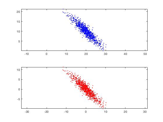
The previous section motivates our reason for using a dimensionality reduction technique. Dimensionality reduction is a type of unsupervised learning where we want to take higher-dimensional data, like images, and represent them in a lower-dimensional space. Let’s use the following image as an example.
These plots show the same data, except the bottom chart zero-centers it. Notice that our data do not have any labels associated with them because this is unsupervised learning! In our simple case, dimensionality reduction will reduce these data from a 2D plane to a 1D line. If we had 3D data, we could reduce it down to a 2D plane or even a 1D line.
All dimensionality reduction techniques aim to find some hyperplane, a higher-dimensional line, to project the points onto. We can imagine a projection as taking a flashlight perpendicular to the hyperplane we’re project onto and plotting where the shadows fall on that hyperplane. For example, in our above data, if we wanted to project our points onto the x-axis, then we pretend each point is a ball and our flashlight would point directly down or up (perpendicular to the x-axis) and the shadows of the points would fall on the x-axis. This is a projection. We won’t worry about the exact math behind this since scikit-learn can apply this projection for us.
In our simple 2D case, we want to find a line to project our points onto. After we project the points, then we have data in 1D instead of 2D! Similarly, if we had 3D data, we want to find a plane to project the points down onto to reduce the dimensionality of our data from 3D to 2D. The different types of dimensionality reduction are all about figuring out which of these hyperplanes to select: there are an infinite number of them!
Princpal Component Analysis
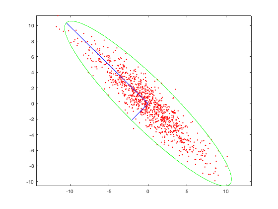
One technique of dimensionality reduction is called principal component analysis (PCA). The idea behind PCA is that we want to select the hyperplane such that when all the points are projected onto it, they are maximally spread out. In other words, we want the axis of maximal variance! Let’s consider our example plot above. A potential axis is the x-axis or y-axis, but, in both cases, that’s not the best axis. However, if we pick a line that cuts through our data diagonally, that is the axis where the data would be most spread!
The longer blue axis is the correct axis! If we were to project our points onto this axis, they would be maximally spread! But how do we figure out this axis? We can borrow a term from linear algebra called eigenvectors! This is where eigenfaces gets its name! Essentially, we compute the covariance matrix of our data and consider that covariance matrix’s largest eigenvectors. Those are our principal axes and the axes that we project our data onto to reduce dimensions. Using this approach, we can take high-dimensional data and reduce it down to a lower dimension by selecting the largest eigenvectors of the covariance matrix and projecting onto those eigenvectors.
Since we’re computing the axes of maximum spread, we’re retaining the most important aspects of our data. It’s easier for our classifier to separate faces when our data are spread out as opposed to bunched together.
(There are other dimensionality techniques, such as Linear Discriminant Analysis, that use supervised learning and are also used in face recognition, but PCA works really well!)
How does this relate to our challenge of face recognition? We can conceptualize our $m\times n$ images as points in $m\dot n$-dimensional space. Then, we can use PCA to reduce our space from $m\dot n$ into something much smaller. This will help speed up our computations and be robust to noise and variation.
Aside on Face Detection
So far, we’ve assumed that the input image is only that of a face, but, in practice, we shouldn’t require the camera images to have a perfectly centered face. This is why we run an out-of-the-box face detection algorithm, such as a cascade classifier trained on faces, to figure out what portion of the input image has a face in it. When we have that bounding box, we can easily slice out that portion of the input image and use eigenfaces on that slice. (Usually, we smooth that slide and perform an affine transform to de-warp the face if it appears at an angle.) For our purposes, we’ll assume that we have images of faces already.
Eigenfaces Code
Now that we’ve discussed PCA and eigenfaces, let’s code a face recognition algorithm using scikit-learn! First, we’ll need a dataset. For our purposes, we’ll use an out-of-the-box dataset by the University of Massachusetts called Labeled Faces in the Wild (LFW).
Feel free to substitute your own dataset! If you want to create your own face dataset, you’ll need several pictures of each person’s face (at different angles and lighting), along with the ground-truth labels. The wider variety of faces you use, the better the recognizer will do. The easiest way to create a dataset for face recognition is to create a folder for each person and put the face images in there. Make sure each are the same size and resize them so they aren’t large images! Remember that PCA will reduce the image’s dimensionality when we project onto that space anyways so using large, high-definition images won’t help and will slow down our algorithm. A good size is ~512×512 for each image. The images should all be the same size so you can store them in one numpy array with dimensions (num_examples, height, width) . (We’re assuming grayscale images). Then use the folder names to disambiguate classes. Using this approach, you can use your own images.
However, we’ll be using the LFW dataset. Luckily, scikit-learn can automatically load our dataset for us in the correct format. We can call a function to load our data. If the data aren’t available on disk, scikit-learn will automatically download them for us from the University of Massachusetts’ website.
import matplotlib.pyplot as plt

from sklearn.model_selection import train_test_split
from sklearn.datasets import fetch_lfw_people
from sklearn.metrics import classification_report
from sklearn.decomposition import PCA
from sklearn.neural_network import MLPClassifier


# Load data
lfw_dataset = fetch_lfw_people(min_faces_per_person=100)

_, h, w = lfw_dataset.images.shape
X = lfw_dataset.data
y = lfw_dataset.target
target_names = lfw_dataset.target_names

# split into a training and testing set
X_train, X_test, y_train, y_test = train_test_split(X, y, test_size=0.3)
The argument to our function just prunes all people without at least 100 faces, thus reducing the number of classes. Then we can extract our dataset and other auxiliary information. Finally, we split our dataset into training and testing sets.
Now we can simply use scikit-learn’s PCA class to perform the dimensionality reduction for us! We have to select the number of components, i.e., the output dimensionality (the number of eigenvectors to project onto), that we want to reduce down to, and feel free to tweak this parameter to try to get the best result! We’ll use 100 components. Additionally, we’ll whiten our data, which is easy to do with a simple boolean flag! (Whitening just makes our resulting data have a unit variance, which has been shown to produce better results)
# Compute a PCA
n_components = 100
pca = PCA(n_components=n_components, whiten=True).fit(X_train)

# apply PCA transformation
X_train_pca = pca.transform(X_train)
X_test_pca = pca.transform(X_test)
We can apply the transform to bring our images down to a 100-dimensional space. Notice we’re not performing PCA on the entire dataset, only the training data. This is so we can better generalize to unseen data.
Now that we have a reduced-dimensionality vector, we can train our neural network!
# train a neural network
print("Fitting the classifier to the training set")
clf = MLPClassifier(hidden_layer_sizes=(1024,), batch_size=256, verbose=True, early_stopping=True).fit(X_train_pca, y_train)
To see how our network is training, we can set the verbose flag. Additionally, we use early stopping.
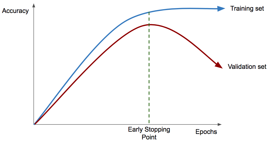
Let’s discuss early stopping as a brief aside. Essentially, our optimizer will monitor the average accuracy for the validation set for each epoch. If it notices that our validation accuracy hasn’t increased significantly for a certain number of epochs, then we stop training. This is a regularization technique that prevents our model from overfitting!
Consider the above chart. We notice overfitting when our validation set accuracy starts to decline. At that point, we immediately stop training to prevent overfitting.
Finally, we can make a prediction and use a function to print out an entire report of quality for each class.
y_pred = clf.predict(X_test_pca)
print(classification_report(y_test, y_pred, target_names=target_names))
Here’s an example of a classification report.
                   precision    recall  f1-score   support

     Colin Powell       0.86      0.89      0.87        66
  Donald Rumsfeld       0.85      0.61      0.71        38
    George W Bush       0.88      0.94      0.91       177
Gerhard Schroeder       0.67      0.69      0.68        26
       Tony Blair       0.86      0.71      0.78        35

      avg / total       0.85      0.85      0.85       342
Notice there is no accuracy metric. Accuracy isn’t the most specific kind of metric to begin. Instead, we see precision, recall, f1-score, and support. The support is simply the number of times this ground truth label occurred in our test set, e.g., in our test set, there were actually 35 images of Tony Blair. The F1-Score is actually just computed from the precision and recall scores. Precision and recall are more specific measures than a single accuracy score. A higher value for both is better.
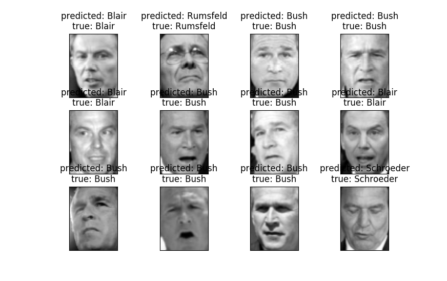
After training our classifier, we can give it a few images to classify.
# Visualization
def plot_gallery(images, titles, h, w, rows=3, cols=4):
    plt.figure()
    for i in range(rows * cols):
        plt.subplot(rows, cols, i + 1)
        plt.imshow(images[i].reshape((h, w)), cmap=plt.cm.gray)
        plt.title(titles[i])
        plt.xticks(())
        plt.yticks(())

def titles(y_pred, y_test, target_names):
    for i in range(y_pred.shape[0]):
        pred_name = target_names[y_pred[i]].split(' ')[-1]
        true_name = target_names[y_test[i]].split(' ')[-1]
        yield 'predicted: {0}\ntrue: {1}'.format(pred_name, true_name)

prediction_titles = list(titles(y_pred, y_test, target_names))
plot_gallery(X_test, prediction_titles, h, w)(plot_gallery and titles functions modified from the scikit-learn documentation)
We can see our network’s predictions and the ground truth value for each image.
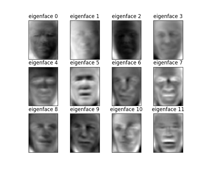
Another thing interesting thing to visualize is are the eigenfaces themselves. Remember that PCA produces eigenvectors. We can reshape those eigenvectors into images and visualize the eigenfaces.
These represent the “generic” faces of our dataset. Intuitively, these are vectors that represent directions in “face space” and are what our neural network uses to help with classification. Now that we’ve discussed the eigenfaces approach, you can build applications that use this face recognition algorithm!
We discussed a popular approach to face recognition called eigenfaces. The essence of eigenfaces is an unsupervised dimensionality reduction algorithm called Principal Components Analysis (PCA) that we use to reduce the dimensionality of images into something smaller. Now that we have a smaller representation of our faces, we apply a classifier that takes the reduced-dimension input and produces a class label. For our classifier, we used a single-layer neural network.
Face recognition is a fascinating example of merging computer vision and machine learning and many researchers are still working on this challenging problem today!
Nowadays, deep convolutional neural networks are used for face recognition, and have vast implications in terms of the development career world. Try one out on this dataset!
