“Data science” or “Big data analyst” is a phrase that has been tossed around since the advent of Big Data. But what is it, really? Well imagine working for a retail company. One of the questions you may be asked to answer is “how many chips should we stock up for this month?” It seems like a simple question that makes sense to ask. But there are a lot of steps involved in answering that single question. We need to collect the data, clean/prep the data, figure out which features we need to answer the question, determine the appropriate machine learning algorithm to use, get the results, and, finally, write a report that outlines the results of the analysis. And that’s still a fairly top-level understanding of what might be needed to complete this task! Some portion of that might take a long time, e.g., we may spend a few weeks collecting and cleaning/prepping data!
We’re going to go through an example question similar to what a data scientist may be expected to answer. We’ll also cover the topic of linear regression, a fundamental machine learning algorithm. Download the dataset and code in the ZIP file here.
Data science hinges on questions whose answer lie in the data itself. We’re going to go through an example of answering one of these questions using data from Facebook. The University of California Irvine (UCI) has a ton of free-to-use machine learning datasets here, and we’re going to use their Facebook metrics dataset to answer some questions.
Let’s start off with a question whose answer you can probably intuit: “When a post is shared more often, do more people tend to like that post as well?” You can probably use your intuition to figure out that the more a post is shared, the more likely it is to be liked or commented on. But intuition doesn’t always pan out! The key word in “data science” is “data”! We need evidence to support our intuition or our hypothesis.
Table of contents
Data Extraction and Exploration
The first thing we should do is spend some time to explore our dataset. This includes writing code to read in our data and to create a visualization. Since the data are in a CSV file, we can use the built-in csv module to extract them. If we’re dealing with large datasets, it’s quicker to pre-allocate our numpy arrays whenever possible. This is why we count the number of rows in our csv file, which should be exactly 500. (We subtract one because of the header row.) Then we can pre-allocate our X and Y arrays. We use Python’s csv module to open the file, skip the header row, and load it into the numpy arrays.
A few minor points to note: the enumerate function will produce a tuple with the index and value at that index if given a list or generator. This is particularly useful for loading into pre-allocated arrays. Another note is that some of data might not exist. In this case, we have to decide what we should do. There are many valid options: forget/remove the nonexistent data, replace it with a default value, interpolate (for time-series data), etc. In our case, we’re just substituting a reasonable value (zero).
import numpy as np
import matplotlib.pyplot as plt
import csv

def load_dataset():
    num_rows = sum(1 for line in open('dataset_Facebook.csv')) - 1
    X = np.zeros((num_rows, 1))
    y = np.zeros((num_rows, 1))
    with open('dataset_Facebook.csv') as f:
        reader = csv.DictReader(f, delimiter=';')
        next(reader, None)
        for i, row in enumerate(reader):
            X[i] = int(row['share']) if len(row['share']) > 0 else 0
            y[i] = int(row['like'])  if len(row['like']) > 0 else 0
    return X, y
Now that our dataset is loaded, we can use matplotlib to create a scatter plot. Remember to label the axes!
def visualize_dataset(X, y):
plt.xlabel('Number of shares')
plt.ylabel('Number of likes')
plt.scatter(X, y)
plt.show()
if __name__ == '__main__':
X, y = load_dataset()
visualize_dataset(X, y)Here is the resulting plot:

From this plot alone, we notice a few things. There seems to be an outlier with around 800 shares and a little over 5000 likes. This might be an interesting post to investigate. A second point to notice is that most of our data are between 0 – 200 shares and 0 – 2000 likes, quite densely actually. Remember that 500 data points are being shown! Another interesting point we notice is the right-upwards trend of our data. This seems to fit our intuition: the more shares a post receives, the most likes it tends to have!
Normally, we would spend more time exploring our data, but our question can be answered using these data. Now that we see our intuition fits our data, we need to provide quantitative numbers that show this relationship between the number of shares and number of likes. The best way to do this, in our case, is using linear regression.
Linear Regression
Linear regression is a machine learning algorithm used find linear relationships between two sets of data. The crux of linear regression is that it only works when our data is somewhat linear, which fits our data. There are metrics that we’ll use to see exactly how linear our data are.
With linear regression, we’re trying to estimate the parameters of a line:
![\[ \hat{y} = wx + b \]](https://gamedevacademy.org/wp-content/ql-cache/quicklatex.com-3948a3969e33ffd642043084f7567f96_l3.png "Rendered by QuickLaTeX.com")
Following suit with neural networks, we use  instead of
  . Another reason for this is because we may have multivariate data where the input is a vector. Then we generalize to a dot product. Based on this equation, we have two parameters: and
  .
.
We want to compute the line-of-best-fit, but what does “best” mean? Well we need to define a metric that we use to measure “best” because we need a way to determine if one set of parameter values is better than another. To do this, we define a cost function. Intuitively, this is just a measure of how good our parameters are, given our data. When our cost function is minimal, that means that our parameters are optimal!

(where N is the number of training examples and y is the true value)
Let’s take a closer look at this cost function intuitively. It is measuring the sum of the squared error of all of our training examples. The reason we square is because we don’t really care if the error is positive or negative: an error is an error! (More precisely, the reason we use a square and not an absolute value is because it is differentiable: the derivative of a squared function is nicer than the derivative of an absolute value function.)
Now that we know a bit about the cost function. How do we use it? The optimal parameters are found when the cost is at a minimum. So we need to perform some optimization! To find the optimal value of w, we take the partial derivative of  with respect to , set it equal to zero, and solve for ! We do the same thing for .
We’ll skip the partial derivatives and derivation for now, but we can use some statistics to rearrange the solutions into a closed-form:

(where the bars over the variables represent average/mean)
Now we can figure out the slope and y-intercept from the data itself!
Linear Regression Code
Now that we have the math figured out, we can implement this in code. Let’s create a new class with parameters w and b.
class LinearRegression(object):
    """Implements linear regression"""
    def __init__(self):
        self.w = 0
        self.b = 0
Now we can write a fit function that computes both of these using the closed-forms we discussed.
def fit(self, X, y):
    mean_x = X.mean()
    mean_y = y.mean()
    errors_x = X - mean_x
    errors_y = y - mean_y
    errors_product_xy = np.sum(np.multiply(errors_x, errors_y))
    squared_errors_x = np.sum(errors_x ** 2)

    self.w = errors_product_xy / squared_errors_x
    self.b = mean_y - self.w * mean_x
We are making use of numpy’s vectorized operations to speed up our computation. We compute the means of our inputs and outputs using a quick numpy function. We can compute the errors in a vectorized fashion as well. In numpy, when we perform addition, subtraction, multiplication, or division of an array by a scalar, numpy will apply that operation to all values in the array. For example, when we subtract the scalar mean_x from the vector X, we’re actually taking each element of X and subtracting mean_x from it. Same goes for the vector y.
When we compute the errors, we have to tell numpy to do an element-wise multiplication of the two vectors, not a vector-vector multiplication. (Mathematically, this is called the Hadamard product). This takes the first element of errors_x and multiplies it by the first element of errors_y and so on to produce a new vector. Then we take the sum of all of the elements in that vector. This produces the numerator of the expression to compute the slope.
To compute the denominator, we can simply take the square of the errors and take the sum. Numpy can also apply exponents to each element of an array. Finally, we can compute the slope and y-intercept!
Before we visualize our answer, let’s make another convenience function that takes in inputs and applies our equation to return predictions.
def predict(self, X):
    return self.w * X + self.b
Now that we have the slope and y-intercept, we can visualize this along with the scatter plot of our data to see if our solution is correct.
def visualize_solution(X, y, lin_reg):
    plt.xlabel('Number of shares')
    plt.ylabel('Number of likes')
    plt.scatter(X, y)

    x = np.arange(0, 800)
    y = lin_reg.predict(x)
    plt.plot(x, y, 'r--')

    plt.show()

if __name__ == '__main__':
    X, y = load_dataset()
    lin_reg = LinearRegression()
    lin_reg.fit(X, y)

    visualize_solution(X, y, lin_reg)
Here, we simply create some x values and apply our line equation to them to produce the red, dashed line. The result is shown below:

We can see that our red, prediction line-of-best-fit fits most of our data! However, there’s another statistical measure that we can compute to give us more information about our line. In particular, it will tell us how linear our data are and the correlation.
Correlation Coefficient
The Pearson correlation coefficient is a number that represents how linear our data are and the relationship between the input and output, namely between the number of shares and the number of likes.
We won’t cover the exact derivation of it, but we can represent it quite simply in statistical terms:

(where  and
and  are the standard deviations of X and Y and
  is the covariance of X and Y)
We can compute the covariance using the following equation
![\[ \sigma_{xy} = \displaystyle\frac{1}{N}\sum_{i=0}^N(x_i - \bar{x})(y_i - \bar{y}) \]](https://gamedevacademy.org/wp-content/ql-cache/quicklatex.com-bfced25c2871e0e2b27a9273b03affd4_l3.png "Rendered by QuickLaTeX.com")
The correlation coefficient is a value from -1 to 1 that represents two thing: the linearity of our data and the correlation between X and Y. A value close to -1 or 1 means that our data is very linear. A value close to 0 means that our data is not linear at all. If the value is positive, then high values of X tend to produce high values of Y and vice-versa. If the value is negative, high values of X tend to produce low values of Y and vice-versa. This is a very powerful metric and essential to answering our question: “are posts that are shared more often receive more likes?”
To compute the value, let’s add another property.
class LinearRegression(object):
    """Implements linear regression"""
    def __init__(self):
        self.w = 0
        self.b = 0
        self.rho = 0
We can compute this value in the fit function when we have the inputs and outputs.
def fit(self, X, y):
    mean_x = X.mean()
    mean_y = y.mean()
    errors_x = X - mean_x
    errors_y = y - mean_y
    errors_product_xy = np.sum(np.multiply(errors_x, errors_y))
    squared_errors_x = np.sum(errors_x ** 2)

    self.w = errors_product_xy / squared_errors_x
    self.b = mean_y - self.w * mean_x

    N = len(X)
    std_x = X.std()
    std_y = y.std()
    cov = errors_product_xy / N
    self.rho = cov / (std_x * std_y)
Now we can add some code in our visualization to show this value in the legend of the plot.
def visualize_solution(X, y, lin_reg):
    plt.xlabel('Number of shares')
    plt.ylabel('Number of likes')
    plt.scatter(X, y)

    x = np.arange(0, 800)
    y = lin_reg.predict(x)
    plt.plot(x, y, 'r--', label='r = %.2f' % lin_reg.rho)
    plt.legend()

    plt.show()

if __name__ == '__main__':
    X, y = load_dataset()
    lin_reg = LinearRegression()
    lin_reg.fit(X, y)

    visualize_solution(X, y, lin_reg)
Notice the label parameter to the plot function. Finally, we can show our plot:

We notice that our data has a correlation coefficient of +0.9, which is close to 1 and positive. This means our data is really linear and the more shares a post gets, the more likes it tends to get too! We’ve answered our question!
There are many more columns to this data set, and I encourage you to explore all of them using scatter plots, histograms, etc. Try to find hidden correlations! (But remember that correlation does not imply causation!)
To summarize, we learned how to answer a data science question using linear regression, which gives us the line-of-best-fit for our data. We use a cost function to mathematically represent what the “best” line is, and we can use optimization to directly solve for the slope and intercept of the line. However, this equation might not be enough. Additionally, we can compute the correlation coefficient to tell us the linearity of our data and the correlation between the inputs and outputs.
Linear regression is a fundamental machine learning algorithm and essential to data science!