Overview Of Machine Learning

Computers are incredibly dumb. They have to be told explicitly what to do in the form of programs. Programs have to account for every possible branch of logic and are specific to the task at hand. If there are any anomalies in the set of inputs, a program might not produce the right output or just crash outright! In many cases, this behavior is acceptable since programs are quite specialized for a particular purpose. However, there many more cases where we want our program to be more general and learn how to accomplish the task after we have given it many examples of how to do the task. This is only a slice of what the field of artificial intelligence is trying to solve.

Artificial intelligence (AI) is a very broad field in computer science whose goal is to build an entity that can perceive and reason about the world as well as, or better than, humans can. Machine Learning is the largest subfield in AI and tries to move away from this explicit programming of machines. Instead of hard-coding all of our computer’s actions, we provide our computers with many examples of what we want, and the computer will learn what to do when we give it new examples it has never seen before.

To introduce the field, we’ll briefly touch on a wide variety of different topics to get a better feel for what they are and how they work. Later, we’ll delve into more detail to discuss really how and why these techniques, algorithms, and architectures work. First we will discuss, in moderate detail, how AI solved problems before the advent of machine learning. Although those algorithms are still used today for other tasks, they have been replaced by more powerful algorithms, and it will be the only time we discuss classical AI. This should set the stage for moving on to more modern approaches of machine learning. We’ll briefly discuss two of the most common types of machine learning: supervised and unsupervised learning. Finally, there will be a bonus section toward the end briefly introducing neural networks, since they are such a hot topic. Later, we will pick apart a neural network to see exactly how they work and write the code to construct, train, and test it from scratch.

Table of contents

Good Old-Fashioned Artificial Intelligence (GOFAI)

Artificial intelligence is certainly not a new development in computer science. The field has actually existed for many decades (since the 1950s!), but, back then, people in that field were solving problems in a different way than the machine learning algorithms used today: their approaches centered around building search algorithms. And this is what we call good old-fashioned artificial intelligence (GOFAI).

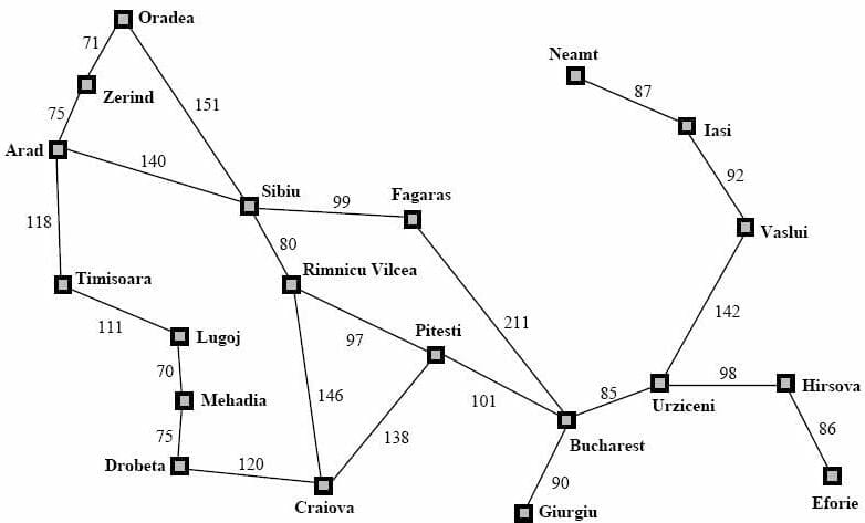
(credit http://athena.ecs.csus.edu/~gordonvs/215/215homework.html)

To illustrate this approach, let’s consider a real-world problem: what’s the best route to go Bucharest from Arad? This is the classic problem that is used to illustrate search algorithms in almost every university course on AI so we’ll also discuss it here. Take a look at the chart above, more formally called a discrete mathematics graph. Each city (or node) is connected to others with an edge. On any edge, we see a number that represents the cost of traveling to a city from a particular city. We can think of this as the distance between them, though the cost can be more generic than that. For our purposes, how this cost value is calculated isn’t important. The goal is to find a list of cities that we can traverse through to find the best, i.e., lowest cost, route to Bucharest.

Suppose we were transported back before modern approaches existed, and we were tasked with writing a program to do this. We won’t cover the variety of search algorithms that exist, but let’s see how we can frame the problem so that we can use search.

(In our case of path planning, we can see how this can be considered a search problem, but it won’t be this obvious for other kinds of problems. If we frame the problem using the components that we’ll discuss, then we can use an off-the-shelf search algorithm to solve our problem.)

From the phrasing of the problem and the map above, we know all of the pieces of information we need to frame our search problem. First of all, the problem statement says that we’re starting in Arad and ending up in Bucharest. These two pieces of information are the start state and goal state. In reality, we may have multiple goal states and thus generalize the notion of goal states to a goal test function, whose job is to test if we’re in a goal state or not. Suppose our goal was to arrive at an airport, and Bucharest, Zerind, and Iasi all had airports. Then arriving at any of these cities would solve our problem!

The other two pieces of information we need to completely frame our search problem are taken from the graph above. Notice that we have a finite, enumerable number of cities. This is called our state space. In our case, the city represents the state, but, consider the example of traveling between two cities of different countries. Then perhaps our state would consist of a tuple of city and country. The state space is simply all states that we’re considering. The other is the successor function. The purpose of this function is to figure out, given one state, the other states can I get to and how much will it cost. This information is encoded in the edges of the graph above. For example, starting in Arad, I can go to Sibiu with a cost of 140.

Now that we have our search problem, we can apply a search algorithm to our problem and get a solution! Typically, we use a data structure to store the states that we’re considering to visit (called the fringe). The data structure, usually a stack, queue, or priority queue, depends on the specific search algorithm. However, all search algorithms follow the same basic steps:

Start at the start state and put it into the data structure
Remove a state from the data structure
Check if it is the goal state. If so, then return!
Figure out what other states we can get to from this state using the successor function.
Put all of those successor states into the data structure
Go to 2

The details of the search algorithm determine how we remove the state from the data structure. For example, if we were doing depth-first search, we would use a stack and pop off the top of the stack. Besides the details of the search algorithm, we can use this framework to return solutions.

To sum up, GOFAI is centered around this notion that we frame a problem using four elements: start state, state space, successor function, and goal states/goal test function, and apply a search algorithm to return the solution.

The Problem with GOFAI

One of the big issues that people had with GOFAI is that these systems weren’t really learning anything. They were searching through a potentially huge state space for the right answer. If we gave a different problem to the same system, it would treat that problem as independent of all of the other problems that system has solved. This isn’t learning!

(credit https://www.pexels.com/search/apple/)

To illustrate this point, think about a child learning what an apple is for the first time. Initially, a child has no idea what this fruit is, but someone tells the child that this is an apple. If you gave a different apple to the child, the child would still tell you that this fruit is an apple. An amazing things happen: the child generalizes the concept of an apple. In other words, you don’t have to show the child every single apple in the world for the child to learn what an apple is; you give the child a few examples and he/she will learn what the abstract concept of an apple is. This is exactly what GOFAI is lacking.

Along comes machine learning, backed by statistics, calculus, linear algebra, and mathematical optimization to save the day! Instead of searching through a state space, we give machine learning algorithms many examples, and they can learn to generalize.

Machine learning algorithms and approaches are characterized by their parameters or weights. These parameters affect the result of the machine learning algorithm. As we give the algorithm more and more examples, the algorithms tune these parameters based on the previous value of the parameters and the examples they’re current looking at. This is an iterative process where we keep feeding in examples and the algorithm keeps tuning parameters until we achieve good results.

Supervised vs Unsupervised Learning

The two largest categories of machine learning are supervised and unsupervised learning. Think back to the example of teaching the child what an apple is. This is a prime example of supervised learning. When teaching the child, we give an example of an apple along with the correct answer: apple. When using supervised learning, we feed the machine learning algorithm an example and the correct answer. This is why we call it supervised learning. Here are just some of the following tasks that supervised learning can help us with.

Image classification: what is in an image, e.g., a cat.
Image captioning: given an image, generate a novel caption that describes it.
Image retrieval: given an image sentence description, fetch the image that most closely represents that description.
Sentiment classification: what is the sentiment behind this phrase?
Machine translation: translating between languages, e.g., English and French.
Curve fitting or predicting trends in business
…

From the list above, supervised learning has many different applications. However, it can be difficult producing labeled datasets. If our problem is very domain-specific, we usually have to hire people to annotate our dataset, which may be costly or time-consuming.

In unsupervised learning, we don’t give the correct answer (often we don’t know it!). Instead, we rely heavily on statistics and the distribution of the input data. Here are some examples of unsupervised learning.

Clustering: given a set of data, we want to find grouping of similar data points.
New example generation: given a set of training data, create a new data point similar to the training data but not actually in the training data
Anomaly detection: find the anomalous data point in a set of data

Compared to supervised learning, we don’t need to spend time and money annotating a dataset. However, the objective of unsupervised learning seems a bit more difficult than supervised learning: we want insights from our data without giving examples of “correct” results.

To summarize, supervised learning requires each example to have a correct answer while unsupervised learning can take a set of unlabeled examples and learn from it. In the future, we’ll learn about various supervised and unsupervised learning algorithms and techniques.

From the examples of supervised and unsupervised classification, we can grasp the essence of machine learning: learning by example. Instead of having to hard-code our programs, we give these algorithms examples of what we want, and they generalize. This is an amazing thing for a computer to do! And we’re going to see exactly how this generalization works across different types of machine learning, modalities (like images, text, audio, etc), and architectures!

BONUS: Neural Networks

As a bonus section, let’s briefly take a look at neural networks. They were invented many decades ago but have recently come to the forefront of machine learning since we have developed new techniques (and even specialized hardware!) to train massive networks.

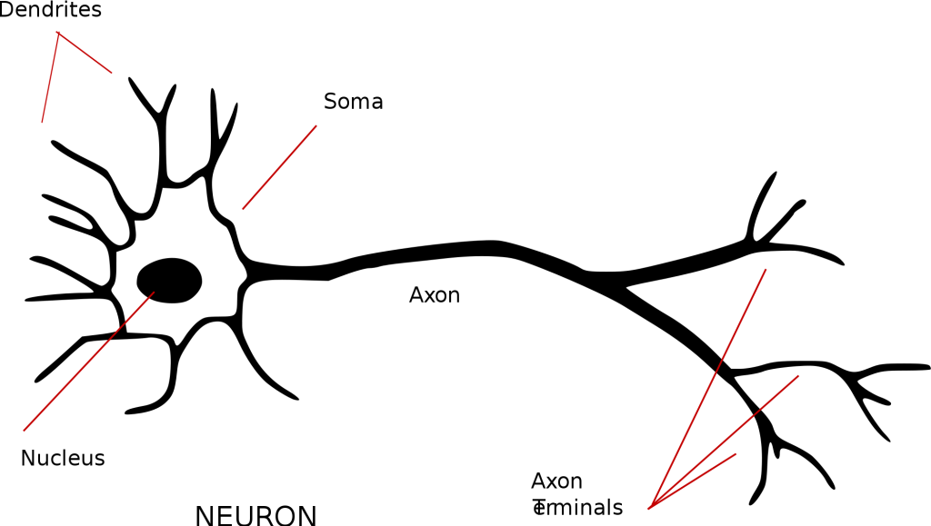
(credit https://commons.wikimedia.org/wiki/File:Neuron_-_annotated.svg)

The inspiration for neural networks comes from biological neurons in our brains. Above is a very simplified version of one. Each neuron takes some number of inputs and produces a single output that may become inputs to other neurons. A biological neuron receives inputs from the dendrites. They touch the cell body, or soma, but, they are connected to other neurons by a little gap called the synapse that weights how strongly this input should be considered. The neuron weights each of its inputs and processes them all together. The actual processing is done in the nucleus. After that processing, the output is sent through the axon so that it may become input to other neurons, and the process repeats.

(credit https://commons.wikimedia.org/wiki/File:Rosenblattperceptron.png)

We can take this biological model and create an approximate, simplified mathematical model from it. The dendrites are the inputs $x_1, ..., x_n$ . We model the synapse as the weights $w_{1j}, ..., w_{nj}$ . Conventionally, the first index refers to the input neuron and the second index refers to the output neuron. In this example, just ignore j (it means the output neuron is the jth neuron in the next layer, but we’ll discuss architecture very soon). We take each input and multiply it with its corresponding weight and add them all up. We’re taking a weighted sum, in other words. Then we apply a non-linear activation function to produce an output. (Later we will see why this function has to be non-linear.) This output $o_j$ , then becomes the input to any number of subsequent neurons.

This is the fundamental model of a single neuron. Surprisingly, a single neuron can still solve a number of different problems. But the recent success of neural networks has come from organizing many of these neurons in connected layers.

(credit http://www.texample.net/tikz/examples/neural-network/)

In the above figure, we have a 2-layer neural network (conventionally, we don’t count the input layer). Each input contributes to each neuron in the hidden layer. Finally, each neuron of the hidden layer goes into the final output layer. This is a very small neural network by today’s standards: many modern architectures are many layers deep and have thousands of neurons per layer.

We’ve seen what a neural network is, but what can they do? Turns out, they can do just about anything! We can use them for both unsupervised and supervised learning. There are special variants of these that work really well for different kinds of inputs like images, text, audio, etc.

We covered a very top-level overview of what neural networks are, but we will discuss them in much more detail. We will discuss different architectures, domain-specific variants, and training algorithms later.