Gaussian Mixture Models are an essential part of data analysis – but do you know how they work?
In this article, we’ll seek to demystify how to analyze “clusters” of data and discuss Gaussian Mixture Models which can help us more efficiently and accurately sort out clusters of data points.
Let’s dive in!
Table of contents
What is Clustering?
Clustering is an essential part of any data analysis. Using an algorithm such as K-Means leads to hard assignments, meaning that each point is definitively assigned a cluster center. This leads to some interesting problems: what if the true clusters actually overlap? What about data that is more spread out; how do we assign clusters then?
Gaussian Mixture Models save the day! We will review the Gaussian or normal distribution method and the problem of clustering. Then we will discuss the overall approach of Gaussian Mixture Models. Training them requires using a very famous algorithm called the Expectation-Maximization Algorithm that we will discuss.
Download the full code here.
If you are not familiar with the K-Means algorithm or clustering, read about it here.
Did you come across any errors in this tutorial? Please let us know by completing this form and we’ll look into it!

FINAL DAYS: Unlock coding courses in Unity, Godot, Unreal, Python and more.
Gaussian Distribution
The first question you may have is “what is a Gaussian?”. It’s the most famous and important of all statistical distributions. A picture is worth a thousand words so here’s an example of a Gaussian centered at 0 with a standard deviation of 1.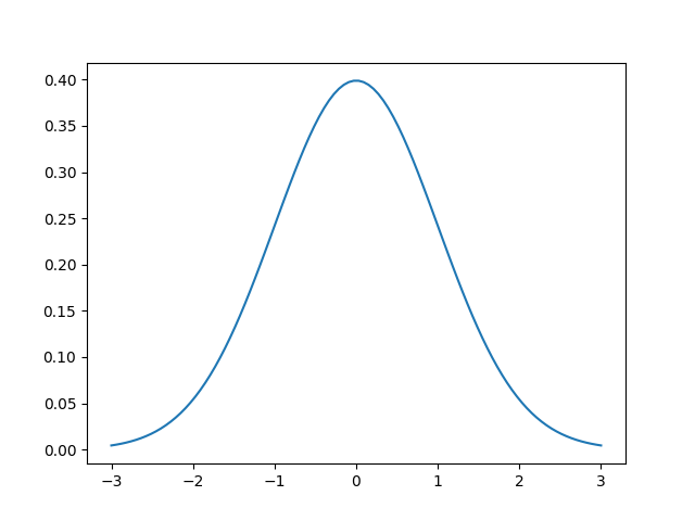
This is the Gaussian or normal distribution! It is also called a bell curve sometimes. The function that describes the normal distribution is the following
\[ \mathcal{N}(x; \mu, \sigma^2) = \displaystyle\frac{1}{\sqrt{2\pi\sigma^2}}e^{-\displaystyle\frac{(x-\mu)^2}{2\sigma^2}} \]
That looks like a really messy equation! And it is, so we’ll use $\mathcal{N}(x; \mu, \sigma^2)$ to represent that equation. If we look at it, we notice there are one input and two parameters. First, let’s discuss the parameters and how they change the Gaussian. Then we can discuss what the input means.
The two parameters are called the mean $\mu$ and standard deviation $\sigma$. In some cases, the standard deviation is replaced with the variance $\sigma^2$, which is just the square of the standard deviation. The mean of the Gaussian simply shifts the center of the Gaussian, i.e., the “bump” or top of the bell. In the image above, $\mu=0$, so the largest value is at $x=0$.
The standard deviation is a measure of the spread of the Gaussian. It affects the “wideness” of the bell. Using a larger standard deviation means that the data are more spread out, rather than closer to the mean.
What about the input? More specifically, the above function is called the probability density function (pdf) and it tells us the probability of observing an input $x$, given that specific normal distribution. Given the graph above, we see that observing an input value of 0 gives us a probability of about 40%. As we move away in either direction from the center, we are decreasing the probability. This is one key property of the normal distribution: the highest probability is located at mean while the probabilities approach zero as we move away from the mean.
(Since this is a probability distribution, the sum of all of the values under the bell curve, i.e., the integral, is equal to 1; we also have no negative values.)
Why are we using the Gaussian distribution? The Expectation-Maximization algorithm is actually more broad than just the normal distribution, but what makes Gaussians so special? It turns out that many dataset distributions are actually Gaussian! We find these Gaussians in nature, mathematics, physics, biology, and just about every other field! They are ubiquitous! There is a famous theorem in statistics called the Central Limit Theorem that states that as we collect more and more samples from a dataset, they tend to resemble a Gaussian, even if the original dataset distribution is not Gaussian! This makes Gaussian very powerful and versatile!
Multivariate Gaussians
We’ve only discussed Gaussians in 1D, i.e., with a single input. But they can easily be extended to any number of dimensions. For Gaussian Mixture Models, in particular, we’ll use 2D Gaussians, meaning that our input is now a vector instead of a scalar. This also changes our parameters: the mean is now a vector as well! The mean represents the center of our data so it must have the same dimensionality as the input.
The variance changes less intuitively into a covariance matrix $\Sigma$. The covariance matrix, in addition to telling us the variance of each dimension, also tells us the relationship between the inputs, i.e., if we change x, how does y tend to change?
We won’t discuss the details of the multivariate Gaussian or the equation that generates it, but knowing what it looks like is essential to Gaussian Mixture Models since we’ll be using these.
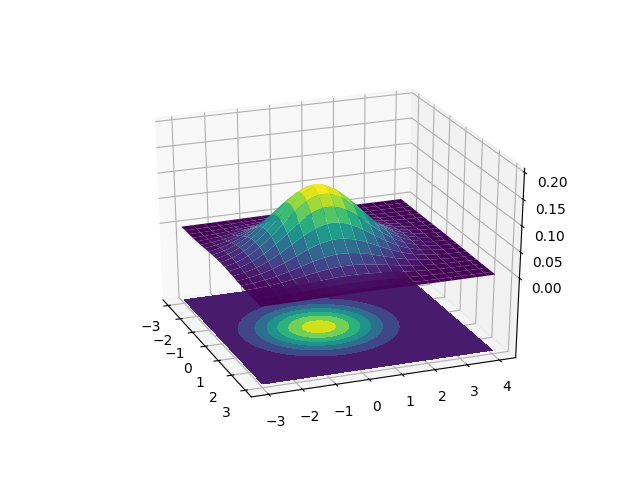
The above chart has two different ways to represent the 2D Gaussian. The upper plot is a surface plot that shows this our 2D Gaussian in 3D. The X and Y axes are the two inputs and the Z axis represents the probability. The lower plot is a contour plot. I’ve plotted these on top of each other to show how the contour plot is just a flattened surface plot where color is used to determine the height. The lighter the color, the larger the probability. The Gaussian contours resemble ellipses so our Gaussian Mixture Model will look like it’s fitting ellipses around our data. Since the surface plot can get a little difficult to visualize on top of data, we’ll be sticking to the contour plots.
Gaussian Mixture Models
Now that we understand Gaussians, let’s discuss to Gaussian Mixture Models (GMMs)! To motivate our discussion, let’s see some example data that we want to cluster.
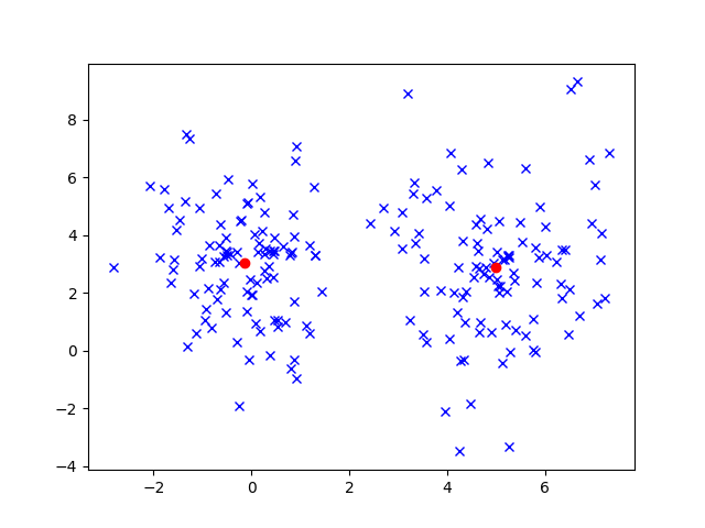
We could certainly cluster these data using an algorithm like K-Means to get the following results.
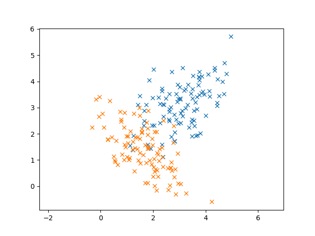
In this case, K-Means works out pretty well. But let’s consider another case where we have overlap in our data. (The two Gaussians are colored differently)
In this case, it’s pretty clear that these data are generated from Gaussians from the elliptical shape of the 2D Gaussian. In fact, we know that these data follow the normal distribution so using K-Means doesn’t seem to take advantage of that fact. Even though I didn’t tell you our data were normally distributed, remember that the Central Limit Theorem says that enough random samples from any distribution will look like the normal distribution.
Additionally, K-Means doesn’t take into account the covariance of our data. For example, the blue points seem to have a relationship between X and Y: larger X values tend to produce larger Y values. If we had two points that were equidistant from the center of the cluster, but one followed the trend and the other didn’t, K-Means would regard them as being equal, since it uses Euclidean distance. But it seems certainly more likely that the point that follows the trend should match closer to the Gaussian than the point that doesn’t.
Since we know these data are Gaussian, why not try to fit Gaussians to them instead of a single cluster center? The idea behind Gaussian Mixture Models is to find the parameters of the Gaussians that best explain our data.
This is what we call generative modeling. We are assuming that these data are Gaussian and we want to find parameters that maximize the likelihood of observing these data. In other words, we regard each point as being generated by a mixture of Gaussians and can compute that probability.
\begin{align}
p(x) = \displaystyle\sum_{j=1}^{k} \phi_j\mathcal{N}(x; \mu_j, \Sigma_j)\\
\displaystyle\sum_{j=1}^{k} \phi_j = 1
\end{align}
The first equation tells us that a particular data point $x$ is a linear combination of the $k$ Gaussians. We weight each Gaussian with $\phi_j$, which represents the strength of that Gaussian. The second equation is a constraint on the weights: they all have to sum up to 1. We have three different parameters that we need to write update: the weights for each Gaussian $\phi_j$, the means of the Gaussians $\mu_j$, and the covariances of each Gaussian $\Sigma_j$.
If we try to directly solve for these, it turns out that we can actually find closed-forms! But there is one huge catch: we have to know the $\phi_j$’s! In other words, if we knew exactly which combination of Gaussians a particular point was taken from, then we could easily figure out the means and covariances! But this one critical flaw prevents us from solving GMMs using this direct technique. Instead, we have to come up with a better approach to estimate the weights, means, covariances.
Expectation-Maximization
How do we learn the parameters? There’s a very famous algorithm called the Expectation-Maximization Algorithm, also called the EM algorithm for short, (written in 1977 with over 50,000 paper citations!) that we’ll use for updating these parameters. There are two steps in this algorithm as you might think: expectation and maximization. To explain these steps, I’m going to cover how the algorithm works at a high level.
The first part is the expectation step. In this step, we have to compute the probability that each data point was generated by each of the $k$ Gaussians. In contrast to the K-Means hard assignments, these are called soft assignments since we’re using probabilities. Note that we’re not assigning each point to a Gaussian, we’re simply determining the probability of a particular Gaussian generating a particular point. We compute this probability for a given Gaussian by computing $\phi_j\mathcal{N}(x; \mu_j, \Sigma_j)$ and normalizing by dividing by $\sum_{q=1}^{k} \phi_q\mathcal{N}(x; \mu_q, \Sigma_q)$. We’re directly applying the Gaussian equation, but multiplying it by its weight $\phi_j$. Then, to make it a probability, we normalize. In K-Means, the expectation step is analogous to assigning each point to a cluster.
The second part is the maximization step. In this step, we need to update our weights, means, and covariances. Recall in K-Means, we simply took the mean of the set of points assigned to a cluster to be the new mean. We’re going to do something similar here, except apply our expectations that we computed in the previous step. To update a weight $\phi_j$, we simply sum up the probability that each point was generated by Gaussian $j$ and divide by the total number of points. For a mean $\mu_j$, we compute the mean of all points weighted by the probability of that point being generated by Gaussian $j$. For a covariance $\Sigma_j$, we compute the covariance of all points weighted by the probability of that point being generated by Gaussian $j$. We do each of these for each Gaussian $j$. Now we’ve updated the weights, means, and covariances! In K-Means, the maximization step is analogous to moving the cluster centers.
Mathematically, at the expectation step, we’re effectively computing a matrix where the rows are the data point and the columns are the Gaussians. An element at row $i$, column $j$ is the probability that $x^{(i)}$ was generated by Gaussian $j$.
\[ W^{(i)}_j} = \displaystyle\frac{\phi_j\mathcal{N}(x^{(i)}; \mu_j, \Sigma_j)}{\displaystyle\sum_{q=1}^{k}\phi_q\mathcal{N}(x^{(i)}; \mu_q, \Sigma_q)} \]
The denominator just sums over all values to make each entry in $W$ a probability. Now, we can apply the update rules.
\begin{align*}
\phi_j &= \displaystyle\frac{1}{N}\sum_{i=1}^N W^{(i)}_j\\
\mu_j &= \displaystyle\frac{\sum_{i=1}^N W^{(i)}_j x^{(i)}}{\sum_{i=1}^N W^{(i)}_j}\\
\Sigma_j &= \displaystyle\frac{\sum_{i=1}^N W^{(i)}_j (x^{(i)}-\mu_j)(x^{(i)}-\mu_j)^T}{\sum_{i=1}^N W^{(i)}_j}
\end{align*}
The first equation is just the sum of the probabilites of a particular Gaussian $j$ divided by the number of points. In the second equation, we’re just computing the mean, except we multiply by the probabilities for that cluster. Similarly, in the last equation, we’re just computing the covariance, except we multiply by the probabilities for that cluster.
Applying GMMs
Let’s apply what we learned about GMMs to our dataset. We’ll be using scikit-learn to run a GMM for us. In the ZIP file, I’ve saved some data in a numpy array. We’re going to extract it, create a GMM, run the EM algorithm, and plot the results!
First, we need to load the data.
import numpy as np
import matplotlib.pyplot as plt
from sklearn.mixture import GaussianMixture

X_train = np.load('data.npy')
Additionally, we can generate a plot of our data using the following code.
plt.plot(X[:,0], X[:,1], 'bx')
plt.axis('equal')
plt.show()
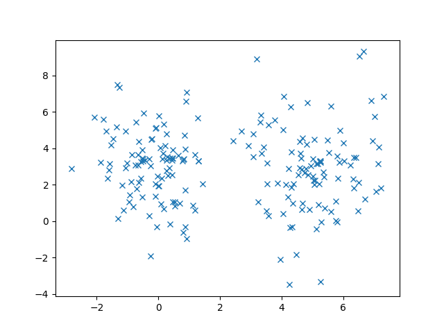
Remember that clustering is unsupervised, so our input is only a 2D point without any labels. We should get the same plot of the 2 Gaussians overlapping.
Using the GaussianMixture class of scikit-learn, we can easily create a GMM and run the EM algorithm in a few lines of code!
gmm = GaussianMixture(n_components=2)
gmm.fit(X_train)
After our model has converged, the weights, means, and covariances should be solved! We can print them out.
print(gmm.means_)
print('\n')
print(gmm.covariances_)
For comparison, I generate the original data data according to the following Gaussians.
\begin{align*}
\mu_1 &= \begin{bmatrix}3 \\ 3\end{bmatrix}\\
\Sigma_1 &=
\begin{bmatrix}
1 & 0.6 \\
0.6 & 1
\end{bmatrix}\\
\mu_2 &= \begin{bmatrix}1.5 \\ 1.5\end{bmatrix}\\
\Sigma_2 &=
\begin{bmatrix}
1 & -0.7 \\
-0.7 & 1
\end{bmatrix}
\end{align*}
Our means should be pretty close to the actual means! (Our covariances might be a bit off due to the weights.) Now we can write some code to plot our mixture of Gaussians.
X, Y = np.meshgrid(np.linspace(-1, 6), np.linspace(-1,6))
XX = np.array([X.ravel(), Y.ravel()]).T
Z = gmm.score_samples(XX)
Z = Z.reshape((50,50))

plt.contour(X, Y, Z)
plt.scatter(X_train[:, 0], X_train[:, 1])

plt.show()
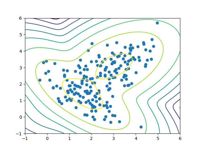
This code simply creates a grid of all X and Y coordinates between -1 and 6 (for both) and evaluates our GMM. Then we can plot our GMM as contours over our original data.
The plot looks just as we expected! Recall that with the normal distribution, we expect to see most of the data points around the mean and less as we move away. In the plot, the first few ellipses have most of the data, with only a few data points towards the outer ellipses. The darker the contour, the lower the score.
(The score isn’t quite a probability: it’s actually a weighted log probability. Remember that each point is generated by a weighted sum of Gaussians, and, in practice, we apply a logarithm for numerical stability, thus prevent underflow.)
To summarize, Gaussian Mixture Models are a clustering technique that allows us to fit multivariate Gaussian distributions to our data. These GMMs well when our data is actually Gaussian or we suspect it to be. We also discussed the famous expectation-maximization algorithm, at a high level, to see how we can iteratively solve for the parameters of the Gaussians. Finally, we wrote code to train a GMM and plot the resulting Gaussian ellipses.
Gaussian Mixture Models are an essential part of data analysis and anomaly detection – which are important to learn when pursuing exciting developer careers! You can also find out more resources for exploring Python here.
