Neural networks have been around for decades, but recent success stems from our ability to successfully train them with many hidden layers. We’ll be opening up the black-box that is deep neural networks and looking at several important algorithms necessary for understanding how they work. To solidify our understanding, we’ll code a deep neural network from scratch and train it on a well-known dataset. Download the full code and dataset here.
Table of contents
Handwritten Digits: The MNIST Dataset
To motivate our discuss of neural networks, let’s take a look at the problem of handwritten digit recognition.
The goal is to determine the correct digit (0-9) given an input. In other words, we want to classify the images into 10 classes, one for each digit. This is more challenging than we may think: each new handwritten digit can have its own little variations, so using a fixed/static representation of a handwritten digit won’t result in a good accuracy. However, machine learning is data-driven, and we can apply it to solve our problem. In particular, we’ll be applying neural networks.
Luckily, we won’t have to go out and collect this data ourselves. In fact, there’s a very famous dataset, colloquially called MNIST, that we’ll be using. In the earlier days, it was used for training the first modern convolutional neural network. It is still sometimes used as a dataset to train on and display results. In fact, there are still challenges to achieve the best accuracy! At the time of this writing, the state-of-the-art result on this dataset is 99.79% accuracy!
I’ve included the dataset in the ZIP file, and the above image is an example taken out of the dataset. To provide more information on the dataset, it consists of binary images of a single handwritten digit (0-9) of size ![]() . The provided training set (the data we use for training our network) has 60,000 images, and the testing set (the data we use for evaluating our network) has 10,000 images. We’ll use it for our neural network and compare our results to the state-of-the-art.
. The provided training set (the data we use for training our network) has 60,000 images, and the testing set (the data we use for evaluating our network) has 10,000 images. We’ll use it for our neural network and compare our results to the state-of-the-art.
Single-layer perceptrons recap
Before we start discuss multilayer perceptrons, if you’re not already familiar with perceptrons, I highly recommending reading this post to acquaint yourself with these models since we will be starting from these small neural networks and adding more complexity.
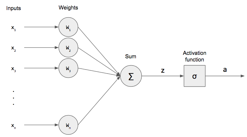
To quickly recap single-layer perceptrons, a neuron had a graphical structure that looked like this.
We take the weighted sum of our input (plus a bias term!) and apply a non-linear activation function. Mathematically, we can write the following statements.

Remember that ![]() is called the pre-activation and
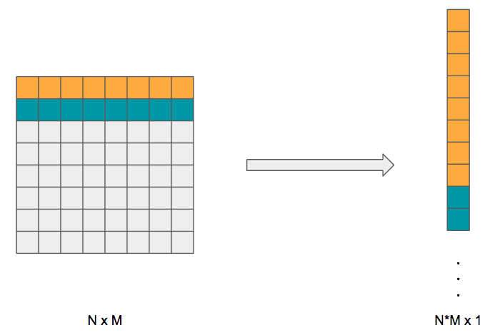
is called the pre-activation and ![]() is the post-activation because we applied the activation function. For our MNIST dataset, we have an image, not an input vector. So how can we convert a 2D image into a 1D vector? We simply flatten it!
is the post-activation because we applied the activation function. For our MNIST dataset, we have an image, not an input vector. So how can we convert a 2D image into a 1D vector? We simply flatten it!
We take the second row of our image and tack it on to the first; we tack on the third row to the concatenation of the first two and so on. What we end up with is a 1D vector representation of our 2D image. This is how we will feed in our inputs into our neural network. Specifically for our MNIST dataset, our images of ![]() are flattened into a single
are flattened into a single ![]() vector, which is the size of our input layer.
vector, which is the size of our input layer.
(The downside to this approach is that we lose spatial information. There is a type of neural network tailored for images called a convolutional neural network where we don’t flatten the input image. These tend to do better at image tasks than regular neural networks.)
Multiple Output Neurons
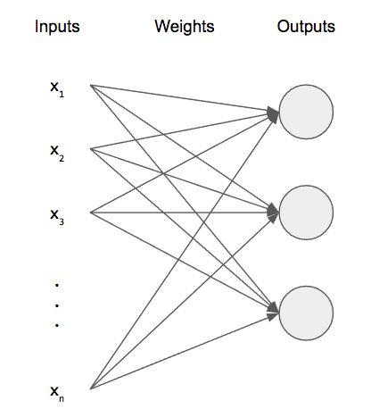
Before we extend this to multiple layers, let’s first extend this to multiple outputs. Right now, we only have a single, scalar output: ![]() . While this is useful for binary classification, it isn’t useful for much else. If we wanted to build a network that can classify more than two classes, we need to add more output neurons. For our MNIST dataset, since we have 10 classes (one for each digit), we’d need 10 output neurons. (For clarity of figure, I’ve only shown 3 output neurons).
. While this is useful for binary classification, it isn’t useful for much else. If we wanted to build a network that can classify more than two classes, we need to add more output neurons. For our MNIST dataset, since we have 10 classes (one for each digit), we’d need 10 output neurons. (For clarity of figure, I’ve only shown 3 output neurons).
Some of the mathematics changes when we do this: the weight vector becomes a weight matrix ![]() with dimensions
with dimensions ![]() , or, more generally,
, or, more generally, ![]() . Additionally, our pre- and post-activations become vectors
. Additionally, our pre- and post-activations become vectors ![]() and
and ![]() . The activation function
. The activation function ![]() is just applied element-wise to each component in vector
is just applied element-wise to each component in vector ![]() . The beauty of this generalization is that we can re-write our equations, and they look almost identical to when we had a single output neuron. We just now have vectors instead of scalars in some places and matrices instead of vectors in other places.
. The beauty of this generalization is that we can re-write our equations, and they look almost identical to when we had a single output neuron. We just now have vectors instead of scalars in some places and matrices instead of vectors in other places.
![]()
(I’ve included the bias explicitly and will continue to do so from here on.)
We can write this in terms of scalars as well. Suppose the input layer is indexed by ![]() and output layer by
and output layer by ![]() , we can re-write the above in component form.
, we can re-write the above in component form.

This is just saying that to get the pre-activation of an arbitrary neuron ![]() in the output layer, we have to take each input, multiply it by the weight that connects that input to that
in the output layer, we have to take each input, multiply it by the weight that connects that input to that ![]() th neuron, and add the bias for that
th neuron, and add the bias for that ![]() th neuron. To convince yourself that this component-wise form is correct, see the above figure and only consider the first output neuron, i.e.,
th neuron. To convince yourself that this component-wise form is correct, see the above figure and only consider the first output neuron, i.e., ![]() . This component form will be useful later on when we discuss backpropagation: we’ll start off by writing the component forms and then vectorize using linear algebra in the code. In general, vectorized code tends to run faster than non-vectorized code because of the myriad of libraries (e.g., numpy!) specializing in vectorized code.
. This component form will be useful later on when we discuss backpropagation: we’ll start off by writing the component forms and then vectorize using linear algebra in the code. In general, vectorized code tends to run faster than non-vectorized code because of the myriad of libraries (e.g., numpy!) specializing in vectorized code.
But how do we structure our data (inputs and ground-truth outputs) for multi-class learning? The input doesn’t change, but we take the ground-truth and encode it as a one-hot vector. We create a vector with the same length as the number of classes and put a single “1” in the position that corresponds to the correct class. Consider our MNIST dataset. If one of our inputs is actually a 4, then our ground-truth vector would be ![]() . The vector is the zero vector, except we have a single “1” in the position of the correct class. (The first position corresponds to the digit zero.) Since the number of output neurons corresponds to the number of classes, the length of our vector is always the same as the number of output neurons.
. The vector is the zero vector, except we have a single “1” in the position of the correct class. (The first position corresponds to the digit zero.) Since the number of output neurons corresponds to the number of classes, the length of our vector is always the same as the number of output neurons.
Multilayer Perceptron Formulation
Now that we know how to account for multiple output neurons, we can finally get to the formulation for our deep neural network, or multilayer perceptron.
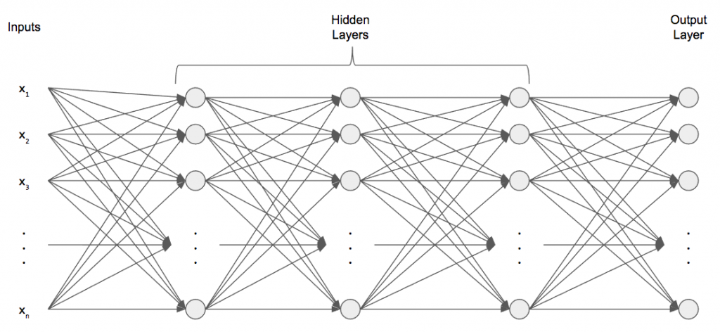
We still have an input and output layer, each with however many neurons we need. But in between those, we have any number of hidden layers, each with any number of neurons. These are called hidden layers because they are not directly connected to the outside world; they are hidden from the outside. Each neuron in a hidden layer is connected to each neuron in the next hidden layer. In the above figure, we have 3 hidden layers, so this is a 4-layer neural network. When we say the number of layers, we exclude the input layer because it really isn’t a “layer” at all. This is also where the deep part of deep neural networks comes in: deep networks have many hidden layers!
So how do these deep neural networks function? They work in an iterative fashion: given an input, we perform the weighted sum (plus bias!) and apply the activation function. For the next hidden layer, we take the post-activations of the layer before it, hidden layer 1, and take the weighted sum (plus bias!) using a different weight matrix and apply the activation function. Then we repeat until we reach the output layer. Neural networks are also called feedforward networks for this exact reason: we feed our input forward through the network. The outputs of a hidden layer become the inputs to the next hidden layer.
Mathematically, we need to add another script for representing which layer we’re referring to.

where ![]() and
and ![]() , i.e., there are L layers. We can, of course, write this is component form as well.
, i.e., there are L layers. We can, of course, write this is component form as well.
We’re not taking exponents; ![]() just means any layer. Also notice that in the pre-activation, we’re no longer just referring to
just means any layer. Also notice that in the pre-activation, we’re no longer just referring to ![]() , but, rather, we take the activation from the previous layer
, but, rather, we take the activation from the previous layer ![]() when computing the pre-activatation of this layer
when computing the pre-activatation of this layer ![]() .
.
Training our Neural Network with Gradient Descent
Now that we’ve formulated and structured our neural network, let’s see how we can train it. To train our neural network, we need some way of quantitatively measuring how well the network, with its current weights and biases, is performing. Just like with single-layer perceptrons, we introduce a cost function that measures the performance of our network. Here’s an example of a cost function.
![]()
where ![]() and
and ![]() represent all of the weights and biases of our network, the sum is over all training examples, and
represent all of the weights and biases of our network, the sum is over all training examples, and ![]() is the activation of the output layer given an input
is the activation of the output layer given an input ![]() .
. ![]() represents the ground-truth label for input
represents the ground-truth label for input ![]() .
.
This is called the quadratic cost or squared error function. Intuitively, we take the squared difference between the network’s answer and the ground-truth answer for each example. If both are vectors, we take the magnitude of the difference.
There are a few properties that all cost functions must follow that this one satisfies. First, it must be strictly greater than 0 everywhere except at a single point. That single point represents the minimum value of ![]() and where the parameters are optimal: they give us a network that can correctly classify everything! Secondly, it must be smooth and differentiable: small differences between the predicted and ground-truth values should translate to a small value for the cost function. If we get a large cost value, that means our network isn’t doing well; if we get a small cost value, then our network is great!
and where the parameters are optimal: they give us a network that can correctly classify everything! Secondly, it must be smooth and differentiable: small differences between the predicted and ground-truth values should translate to a small value for the cost function. If we get a large cost value, that means our network isn’t doing well; if we get a small cost value, then our network is great!
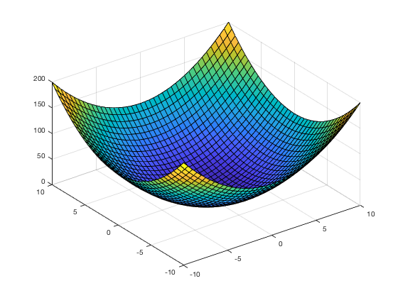
Why do we choose a quadratic cost? Why not a cubic or quartic or some other power? Quadratic functions look like parabolas and have a single global minimum. We can’t say that of other powers (cubic, quartic, etc.). Using a quadratic-like function of two variables, we get a surface that looks kind of like this, where the x and y axes are parameters the z axis (upwards) is the value of the cost function.
Now that we have a way to quantify our network’s performance with the cost function, we can apply the principle of gradient descent to train our network. For now, let’s just consider a cost function with two variable ![]() like the one shown above. We will later apply this princple to our neural network. Since the cost function tells us how well our network is doing, it makes sense to want to minimize this function cost. How do we minimize a function? Calculus! We could use calculus to find the partial derivatives and solve for the minimum. This will work for cost functions with a small number of variables, but, in most cases, neural networks have hundreds, thousands, or millions of parameters! So we have to think of something else.
like the one shown above. We will later apply this princple to our neural network. Since the cost function tells us how well our network is doing, it makes sense to want to minimize this function cost. How do we minimize a function? Calculus! We could use calculus to find the partial derivatives and solve for the minimum. This will work for cost functions with a small number of variables, but, in most cases, neural networks have hundreds, thousands, or millions of parameters! So we have to think of something else.
There is a better way we can find the minimum value, and I’ll explain it using an analogy. Imagine we’re at a point on that quadratic surface in the above figure, and we’re wearing a blindfold so we can’t just see where the valley is and go right to there. How could we find the minimum? We could take a small step around where we are to find which direction the slope goes downhill. The we take a small step in that direction. Then, at that new point, we do the same thing: feel around for the direction that brings us downward and take a small step. We repeat this process until we reach the minimum.
We can solidify this analogy using calculus.
![]()
Intuitively, the change in the cost function is equal to how much we changed ![]() times how much the cost function changes with respect to
times how much the cost function changes with respect to ![]() plus how much we changed
plus how much we changed ![]() times how much the cost function changes with respect to
times how much the cost function changes with respect to ![]() . The partial derivatives tell us how much changing one parameter affects the cost function. The goal is to change
. The partial derivatives tell us how much changing one parameter affects the cost function. The goal is to change ![]() and
and ![]() so that
so that ![]() is negative, therefore we keep moving towards the minimum cost.
is negative, therefore we keep moving towards the minimum cost.
In the analogy, we actually move to a new location on the surface, which called the parameter space. Going to that new position means we change our parameter values. This corresponds to updating the parameter values to reflect that small step. Like in our analogy, we want to take a small step downhill based on where we are locally. How do we know which direction is downhill in calculus? We can use the gradient to do this! The gradient is a vector that always points in the direction of increasing function value. We denote the gradient with an upside-down triangle ![]() called a nabla. More concretely, the gradient is the vector of partial derivatives of each of the parameters:
called a nabla. More concretely, the gradient is the vector of partial derivatives of each of the parameters: ![]() since
since ![]() is a function of two variables. This gradient is a vector that tells us where to go to increase the cost. Since we want to decrease the cost, we can move in the opposite direction of the gradient to get to a lower cost value.
is a function of two variables. This gradient is a vector that tells us where to go to increase the cost. Since we want to decrease the cost, we can move in the opposite direction of the gradient to get to a lower cost value.
![]()
![]() is called the learning rate and represents our step size. It is a hyperparameter, meaning that it isn’t trained by our network: we choose it manually. We can re-write this as a parameter update rule.
is called the learning rate and represents our step size. It is a hyperparameter, meaning that it isn’t trained by our network: we choose it manually. We can re-write this as a parameter update rule.

Our entire analogy is represented in those update equations above. Going back to neural networks, we can apply the same concept of gradient descent. In our case, we have weights and biases. We can write update rules for our weights and biases.

Now we have equations that tell us how to update our neural network’s parameters by going in the opposite direction of the gradient! For each input, we compute the gradient (namely ![]() and
and ![]() ) and sum them all up. Only then can we apply these update rules!
) and sum them all up. Only then can we apply these update rules!
We’ve discussed every term in our update rules except for the two key terms: ![]() and
and ![]() . How do we figure out what these are? To do this, we’ll need to devise the backpropagation of errors algorithm, the most important algorithm for training deep neural networks. We use it to compute the partial derivative of the cost function with respect to every parameter in every layer. We’ll delve into the details next time.
. How do we figure out what these are? To do this, we’ll need to devise the backpropagation of errors algorithm, the most important algorithm for training deep neural networks. We use it to compute the partial derivative of the cost function with respect to every parameter in every layer. We’ll delve into the details next time.
To recap, we learned about the handwritten digits dataset called MNIST (and many of our examples were tailored for that dataset to help solidify abstraction). We extended our perceptron from a single output to multiple output neurons by changing our weight vector to a weight matrix and our output scalar to an output vector. Then we defined the structure of multilayer perceptrons and some notation. Finally, we discussed the fundamental optimization algorithm for neural networks: gradient descent. We always step the parameters in the opposite direction of the gradient to minimize our cost function and train our neural network.
In the subsequent post, we’ll see how to compute the gradient efficiently using the backpropagation of errors, or backprop, algorithm.
Read Part 2 here.

