Read Part 1 here.
Last time, we formulated our multilayer perceptron and discussed gradient descent, which told us to update our parameters in the opposite direction of the gradient. Now we’re going to mention a few improvements on gradient descent and discuss the backpropagation algorithm that will compute the gradients of the cost function so we can update our parameters. Download the full code and dataset here.
Table of contents
Improvements on Gradient Descent
Before moving on to backpropagation, let’s discuss one point of practicality with gradient descent. Recall in vanilla gradient descent (also called batch gradient descent), we took each input in our training set, ran it through the network, computed the gradient, and summed all of the gradients for each input example. Only then did we apply the update rules. But if we have a large training set, we still have to wait to run all inputs before we can update our parameters, and this can take a long time!
Instead, we can take a randomly-sampled subset of our training data to represent the entire training set. For example, instead of running all 60,000 examples of MNIST through our network and then updating our parameters, we can randomly sample 100 examples and run that random sample through our network. That’s a speedup factor of 600! However, we also want to make sure that we’re using all of the training data. It wouldn’t be a good use of the training set if we just randomly sampled 100 images each time. Instead, we randomly shuffle our data and divide it up into minibatches. At each minibatch, we average the gradient and update our parameters before moving on to the next minibatch. After we’ve exhausted all of our minibatches, we say one epoch has passed. Then we shuffle our training data and repeat!
This technique is called minibatch stochastic gradient descent. Mathematically, we can write it like this.

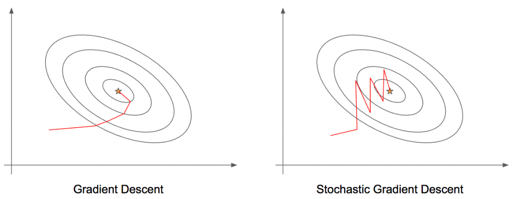
The sum is over all of the samples in our minibatch of size ![]() . The batch size is another hyperparameter: we set it by hand. If we set it too large, then our network will take a longer time to train because it will be more like batch gradient descent. If we set it small, then the network won’t converge. Speaking of convergence, here’s a visual representation of (batch) gradient descent versus (minibatch) stochastic gradient descent.
. The batch size is another hyperparameter: we set it by hand. If we set it too large, then our network will take a longer time to train because it will be more like batch gradient descent. If we set it small, then the network won’t converge. Speaking of convergence, here’s a visual representation of (batch) gradient descent versus (minibatch) stochastic gradient descent.
In this plot, the axes represent the parameters, and the ellipses are cost regions where the star is the minimum. Think of this as a 2D representation of a 3D cost function (see Part 1’s surface plot). Each bend in the line represents a point in the parameter space, i.e., a set of parameters. The goal is to get to the star, the minimum. With gradient descent, the path we take to the minimum is fairly straightforward. However, with stochastic gradient descent, we take a much noisier path because we’re taking minibatches, which cause some variation. That being said, stochastic gradient descent converges, i.e., reaches the minimum (or around there), much faster than gradient descent.
Here’s an algorithm that describes minibatch stochastic gradient descent. We can repeat this algorithm for however many epochs we want.
- Shuffle the training set and split into minibatches of size
 . There will be
  minibatches of size
  where
where  is the ceiling operator.
 - For each minibatch
 :
: - Run
 through our network to and compute the average gradient, i.e.,
  and
and 
- Update the network’s parameters
To recap, stochastic gradient descent drastically improves the speed of convergence by randomly selecting a batch to represent the entire training set instead of looking through the entire training set before updating the parameters.
Minibatch Stochastic Gradient Descent Code
Let’s get to some code! First, we can start by creating a class for our multilayer perceptron. We’ll need to pass in the number of layers and size of each layer as a list of integers. We also define the activation function to be a sigmoid function, but we’ll discuss the details of the activation function a bit later. The exact activation function we choose is unimportant at this point since our algorithms will be generalizable to any activation function.
class MultilayerPerceptron(object):
    """Implementation of a MultilayerPerceptron (MLP)"""
    def __init__(self, layers):
        self.layers = layers
        self.num_layers = len(layers)
        self.activation_fn = sigmoid
        self.d_activation_fn = d_sigmoid

        self.weights = [np.random.randn(y, x) / np.sqrt(x) for x, y in zip(layers[:-1], layers[1:])]
        self.biases = [np.random.randn(y, 1) for y in layers[1:]]
Then we initialize our weights and biases for each layer. Remember that each layer has a different number of neurons and thus requires a different weight matrix and bias vector for each.
One additional heuristic is to initialize the parameters to small, random numbers. Why don’t we just initialize all of them to be the same number like one or zero? Think back to the structure of a neural network. To compute the input into the first hidden layer, we take the weighted sum of the weights and the input. If all of the weights were one, then each hidden neuron receives the same value: the sum of all of the components of the input. This defeats the purpose of having multiple neurons in the hidden layers! Instead, initialize to small, random numbers to break the symmetry. There are more sophisticated ways to initialize our weights and biases, but initializing them randomly works well.
Now we can define a few useful functions that can take an input X, where each row is a training vector, and feed it forward through network. In the case of MNIST and for the purpose of training, X is a matrix of size ![]() because our minibatch size is
because our minibatch size is ![]() and our flattened images are of size 784. The function is general enough to accept minibatches of any size. We iterate through all of the weights and biases of our network and perform
and our flattened images are of size 784. The function is general enough to accept minibatches of any size. We iterate through all of the weights and biases of our network and perform ![]() . Note that
. Note that ![]() starts off as
starts off as ![]() but is then updated in the innermost loop so that we’re always referring to the activation of the previous layer.
but is then updated in the innermost loop so that we’re always referring to the activation of the previous layer.
def feedforward(self, X):
    activations = np.zeros((len(X), self.layers[-1]))
    for i, x in enumerate(X):
        a = x.reshape(-1, 1)
        for W, b in zip(self.weights, self.biases):
            a = self.activation_fn(W.dot(a) + b)
        activations[i] = a.reshape(-1)
    return activations

def accuracy(self, y, pred):
    return np.sum(np.argmax(y, axis=1) == np.argmax(pred, axis=1)) / len(y)
Additionally, we define a helper function that converts the one-hot vector into a number that we can use to compute the accuracy.
Now that we have those functions defined, let’s get to implementing minibatch stochastic gradient descent. At the start of each epoch, we shuffle our training data and divide it up into minibatches. Then, for each minibatch except the last one, we call a function to update our parameters.
def fit(self, X, y, epochs=100, batch_size=100, lr=1e-4):
    N = len(y)
    for e in range(epochs):
        # shuffle and batch
        idx = np.random.permutation(N)
        shuffled_X, shuffled_y = X[idx], y[idx]
        batches = [zip(shuffled_X[b:b+batch_size], shuffled_y[b:b+batch_size]) for b in range(0, N, batch_size)]

        for i in range(len(batches)-1):
            X_train_batch, y_train_batch = zip(*batches[i])
            self.update_params(X_train_batch, y_train_batch, lr)

        X_val_batch, y_val_batch = zip(*batches[-1])
        y_val_batch = np.array(y_val_batch)
        pred_val_batch = self.feedforward(X_val_batch)
        val_accuracy = self.accuracy(y_val_batch, pred_val_batch)
        print("Epoch {0}: Validation Accuracy: {1:.2f}".format(e+1, val_accuracy))
Note that we update parameters for all of the batches except one! For this last batch, we compute the accuracy to act as a kind of “measure of progress” for our network. This is often called the validation set.
Let’s take a look at how we update the parameters. nabla_W and nabla_b represent the total update for all of the weights and biases for this minibatch. In the loop, we accumulate the gradients so that we can apply the update rule in the last few lines of code. We average over the size of the training batch and multiply by the step size or learning rate.
def update_params(self, X_train_batch, y_train_batch, lr):
    nabla_W = [np.zeros_like(W) for W in self.weights]
    nabla_b = [np.zeros_like(b) for b in self.biases]

    for x, y in zip(X_train_batch, y_train_batch):
        delta_nabla_W, delta_nabla_b = self.backprop(x, y)
        nabla_W = [dnW + nW for nW, dnW in zip(delta_nabla_W, nabla_W)]
        nabla_b = [dnb + nb for nb, dnb in zip(delta_nabla_b, nabla_b)]

    self.weights = [W - (lr * nW / len(X_train_batch)) for W, nW in zip(self.weights, nabla_W)]
    self.biases = [b - (lr * nb / len(X_train_batch)) for b, nb in zip(self.biases, nabla_b)]
The most important step happens in the backprop function. This is where we compute the gradient for all of the weights and biases for an example.
Backpropagation
(The notation I use is consistent with Michael Nielsen in his book Neural Networks and Deep Learning.)
Now we can finally discuss backpropagation! It is the fundamental and most important algorithm for training deep neural networks. To start our discuss of backpropagation, remember these update equations.

The ultimate goal is to solve for the partial derivatives of the cost function so we can update our parameters. Can’t we just use calculus to solve for these? Well the answer isn’t quite that simple. The problem is that each parameter isn’t directly connected to the cost function. Consider a weight value connecting the input to the first hidden layer. It isn’t directly connected to the cost function, but the value of the cost function does depend on that weight, i.e., it is a function of that weight (and every weight and bias in the network). So in order to update that weight in the earlier layers, we have to pass backwards through the later layers since the cost function is closer to the weights and biases towards the end. Hence the name backpropagation. Going backwards through the layers corresponds to using the chain rule from calculus, and we’ll see more concrete examples of it.
To make our lives easier, let’s introduce an intermediary term called ![]() and define it like this.
and define it like this.
![Rendered by QuickLaTeX.com \[\delta_j^{(l)} \equiv \displaystyle\frac{\partial C}{\partial z_j^{(l)}} \]](https://gamedevacademy.org/wp-content/ql-cache/quicklatex.com-aecc35bba1524bd857403c02e31acfea_l3.png)
Intuitively, this represents how much changing a particular pre-activation (as a result of a change in a weight or bias) affects the cost function. We’ll call this the local error gradient. Now the only measure of quality of our network is at the very end: the cost function. So to start backpropagation, we need to figure out ![]() (suppose the output neurons are indexed by
(suppose the output neurons are indexed by ![]() ).
).
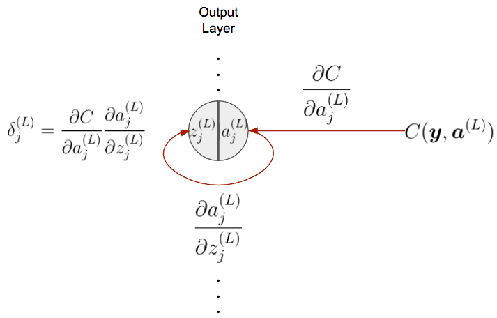
Consider any neuron ![]() in the output layer. The cost function is directly a function of that neuron. We need to go backwards through our network, and that corresponds to taking a derivative! So to go back through the cost function to a particular neuron
in the output layer. The cost function is directly a function of that neuron. We need to go backwards through our network, and that corresponds to taking a derivative! So to go back through the cost function to a particular neuron ![]() , we take the derivative
, we take the derivative ![]() . But this lands us at the post-activation
. But this lands us at the post-activation ![]() , and we need to get to the pre-activation. So we take another derivative to go from post-activation to pre-activation:
, and we need to get to the pre-activation. So we take another derivative to go from post-activation to pre-activation: ![]() . Now we can compute
. Now we can compute ![]() by multiplying these derivatives together! In calculus, this is called the chain rule, and it is essential to backpropagation.
by multiplying these derivatives together! In calculus, this is called the chain rule, and it is essential to backpropagation.
When we solve equation, we get the following.
(1) 
This is the first equation of backpropagation: computing the local error gradient at the last layer! Now that we have the last layer’s local error gradient, we need an equation that tells us how to propagate that error gradient backwards.
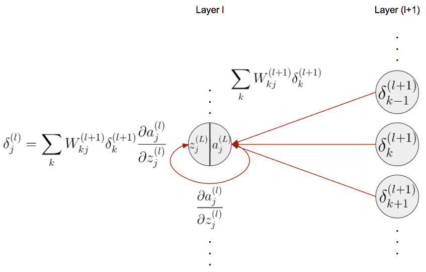
Consider a neuron ![]() in hidden layer
in hidden layer ![]() and all of the neurons, indexed by
and all of the neurons, indexed by ![]() in hidden layer
in hidden layer ![]() . We don’t have to consider the
. We don’t have to consider the ![]() th layer’s pre or post-activations since we’ve already backpropagated through them to get the all of the
th layer’s pre or post-activations since we’ve already backpropagated through them to get the all of the ![]() so we can use those as the starting point. To backprop through the weight matrix, we flip what index we sum over. Since we’re going to a layer indexed by
so we can use those as the starting point. To backprop through the weight matrix, we flip what index we sum over. Since we’re going to a layer indexed by ![]() from a layer indexed by
from a layer indexed by ![]() , we flip the index in the summation to sum over all of the neurons in layer
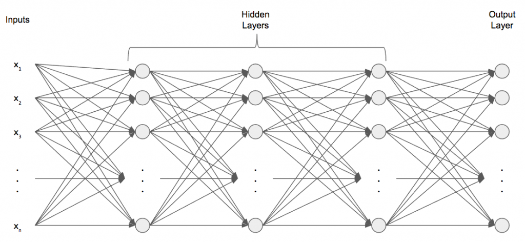
, we flip the index in the summation to sum over all of the neurons in layer ![]() . Looking at the diagram, this makes sense because neuron
. Looking at the diagram, this makes sense because neuron ![]() is connected to all neurons in the
is connected to all neurons in the ![]() th layer. After doing that, we land at the post-activation of layer
th layer. After doing that, we land at the post-activation of layer ![]() . Almost there! We can use the same trick in the previous equation with the partial derivative.
. Almost there! We can use the same trick in the previous equation with the partial derivative.
After expanding this equation, we get the following.
(2) ![]()
Excellent! We’re almost there! Now that we have a way to backpropagate our errors, we can use this local error gradient to calculate the partial derivatives of the weights and biases at a given layer. This is the entire point of backpropagation! Unfortunately, there’s no clever graphic we can refer to; we can directly use the chain rule to figure out the partial derivatives.
(3) 
We’ve finally accomplished our goal! Now we can compute the gradient of the cost function with respect to each weight and bias at each layer! Now let’s write down backpropagation as an algorithm and convert the algorithm to code.
- Feed the input
 through the network and compute each
  and
and  for
for ![Rendered by QuickLaTeX.com l\in[2, L]](data:image/png;base64,iVBORw0KGgoAAAANSUhEUgAAAEAAAAASAQAAAADDVOWPAAAAAnRSTlMAAHaTzTgAAAAMSURBVAjXY2AY7AAAAKIAAcrCDHsAAAAASUVORK5CYII=) .
. - Compute the error at the output layer using
 .
. - For each
![Rendered by QuickLaTeX.com l\in[L-1, 2]](data:image/png;base64,iVBORw0KGgoAAAANSUhEUgAAAF8AAAASAQAAAAAV8T/qAAAAAnRSTlMAAHaTzTgAAAAMSURBVAjXY2AYKQAAAOoAASpuYC8AAAAASUVORK5CYII=)
- Compute the local error gradient
 .
. - Compute the weight gradient
 and bias gradient
  .
.
After we computed the gradients, we can apply gradient descent to update our weights and biases.
Backpropagation Code
Let’s see what backpropagation looks like in code. Note the first step is to feed forward an input; the reason we can’t use the feedforward function is because we need to cache the pre and post-activations so we can use them in the backward pass. The rest of this function is solidifies the mathematics into numpy code. We first compute ![]() and
and ![]() , then we iterate through our layers backwards and use the formulas to compute
, then we iterate through our layers backwards and use the formulas to compute ![]() and
and ![]() for each weight and bias in our network.
for each weight and bias in our network.
def backprop(self, x, y):
    nabla_W = [np.zeros(W.shape) for W in self.weights]
    nabla_b = [np.zeros(b.shape) for b in self.biases]

    # forward pass
    a = x.reshape(-1, 1)
    activations = [a]
    zs = []
    for W, b in zip(self.weights, self.biases):
        z = W.dot(a) + b
        zs.append(z)
        a = self.activation_fn(z)
        activations.append(a)

    # backward pass
    nabla_C = d_cost(y.reshape(-1, 1), activations[-1])
    delta = np.multiply(nabla_C, self.d_activation_fn(zs[-1]))
    nabla_b[-1] = delta
    nabla_W[-1] = delta.dot(activations[-2].T)

    for l in range(2, self.num_layers):
        z = zs[-l]
        delta = np.multiply(self.weights[-l+1].T.dot(delta), self.d_activation_fn(z))
        nabla_b[-l] = delta
        nabla_W[-l] = delta.dot(activations[-l-1].T)
    return (nabla_W, nabla_b)
Note that I’ve vectorized the backprop equations to take full advantage of numpy. One extra thing we need is the derivative of the cost function with respect to the activation. Using the same quadric cost function, we can take the derivative to simply get the difference of the activation and ground-truth value.
def d_cost(y, pred):
    return pred - y
Let’s have a brief aside about the activation function. We’ve abstracted away the activation function, but, for backprop, we need to supply one and its derivative. We’ve seen the activation function for single-layer perceptrons, but it doesn’t work too well for multilayer perceptrons. The reason is because of that pesky threshold. If we made a small change, we could get a completely different output! Instead, we want a smoother activation function: small changes to the inputs should result in small changes to the output so we know we’re on the right track.
We can take that threshold function and smooth it out. The result is what we call a logistic sigmoid, or sigmoid, for short. The sigmoid is defined by this equation
![]()
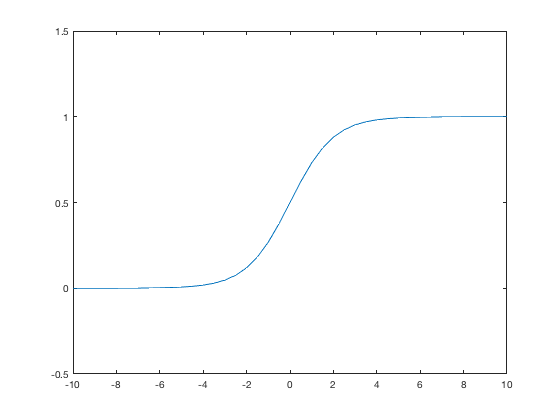
If we plot it, it looks like this.
The sigmoid has several nice properties: it acts as a squashing function by taking its input and squashing it between zero and one; is smooth and differentiable; and a small ![]() results in a small
results in a small ![]() .
.
In code, we can write the sigmoid and its derivative like this.
def sigmoid(z):
    return 1.0 / (1 + np.exp(-z))
def d_sigmoid(z):
    return sigmoid(z) * (1 - sigmoid(z))
In the past few years, sigmoids have fallen out of practice since they saturate for high and low inputs, meaning the derivative of the sigmoid is very small. Take a look at the ends of the sigmoid: the slope hardly changes at all! Instead, researchers have favored a new activation function called a Rectified Linear Unit or ReLU for short.
We can use our new class very simply like this:
if __name__ == '__main__':
    X_train, y_train, X_test, y_test = load_mnist()

    # 2 layer network: 784 input layer, 512 hidden layer, and 10 output layer
    mlp = MultilayerPerceptron(layers=[784, 512, 10])
    mlp.fit(X_train, y_train)

    pred = mlp.predict(X_test)
    accuracy = mlp.accuracy(y_test, pred)
    print("Test accuracy: {0:.2f}".format(accuracy))
The MNIST dataset and code to load MNIST is in the ZIP file!
Here’s some output running for only 10 epochs with a batch size of 128.
Epoch 1: Validation Accuracy: 0.07
Epoch 2: Validation Accuracy: 0.08
Epoch 3: Validation Accuracy: 0.14
Epoch 4: Validation Accuracy: 0.14
Epoch 5: Validation Accuracy: 0.15
Epoch 6: Validation Accuracy: 0.19
Epoch 7: Validation Accuracy: 0.29
Epoch 8: Validation Accuracy: 0.30
Epoch 9: Validation Accuracy: 0.27
Epoch 10: Validation Accuracy: 0.30
Test accuracy: 0.32
To recap, we discussed an improvement on gradient descent called minibatch stochastic gradient descent. Instead of performing an update after seeing every example, we divide our training set into randomly sampled minibatches and update our parameters after computing the gradient averaged across that minibatch. We keep going until all of the minibatches have been seen by the network, then we shuffle our training set and start over! Next, we discussed the fundamental and most important algorithm for training deep neural networks: backpropagation! Using this algorithm, we can compute the gradient of the cost function for each parameter in our network, regardless of the network’s size!
Backpropagation and Gradient Descent are the two of the most important algorithms for training deep neural networks and performing parameter updates, respectively. A solid understanding of both are crucial to your deep learning success.
 and
and 
