Understanding Advanced Convolutional Neural Networks

Convolutional Neural Networks (CNNs) are used in all of the state-of-the-art vision tasks such as image classification, object detection and localization, and segmentation. Previously, we’ve only discussed the LeNet-5 architecture, but that hasn’t been used in practice for decades! We’ll discuss some more modern and complicated architectures such as GoogLeNet, ResNet, and DenseNet. These are the state-of-the-art networks that won challenges such as the ImageNet Large Scale Visual Recognition Challenge (ILSVRC), CIFAR-10, and CIFAR-1000.

If you are not familiar with convolutional neural networks, please see our introduction here.

Did you come across any errors in this tutorial? Please let us know by completing this form and we’ll look into it!

FREE COURSES

FINAL DAYS: Unlock coding courses in Unity, Godot, Unreal, Python and more.

ACCESS FOR FREE

Table of contents

AlexNet

The paper that started the entire deep learning craze: ImageNet Classification with Deep Convolutional Neural Networks by Alex Krizhevsky, Ilya Sutskever, and Geoffrey E. Hinton. AlexNet showed that we can efficiently train deep convolutional neural networks using GPUs.

Source (ImageNet Classification with Deep Convolutional Neural Networks by Alex Krizhevsky, Ilya Sutskever, and Geoffrey E. Hinton) (Fun fact: the figure is taken from the actual paper and is actually cut off!)

AlexNet uses model parallelism to split the network across multiple GPUs. The architecture uses 4 groupings of convolutional, activation, and pooling layers, and 3 fully-connected layers of 4096, 4096, and 1000, where the output vector has a dimensionality of 1000.

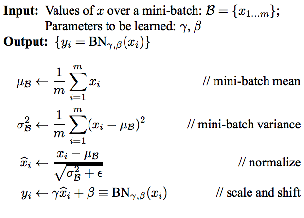
However, we also use an additional layer called a Batch Normalization layer. The motivation behind it is purely statistical: it has been shown that normalized data, i.e., data with zero mean and unit variance, allows networks to converge much faster. So we want to normalize our mini-batch data, but, after applying a convolution, our data may not still have a zero mean and unit variance anymore. So we apply this batch normalization after each convolutional layer.

The implementation of Batch Normalization itself is pretty straightforward.

Source (Batch Normalization: Accelerating Deep Network Training by Reducing Internal Covariate Shift by Sergey Ioffe and Christian Szegedy)

There are two parameters to this batch normalization layer: $\gamma$ and $\beta$ . We compute two quantities: the mean over the batch and the variance over the batch. Each input $x_i$ is actually a vector (technically, a tensor). Hence, the mean and variance are also tensors. After computing these quantities, we have a normalization step where we shift each point so it has a zero mean and unit variance. The $\varepsilon$ is just a small constant added for numerical stability. Then, we apply two transforms: scaling by $\gamma$ and shifting by $\beta$ . These values are learned by the network during the backward pass. When introducing this new layer into our network, we have to backpropagate through it. Certainly batch normalization can be backpropagated over, and the exact gradient descent rules are defined in the paper.

Since we apply batch normalization after each convolution, our AlexNet architecture is now 4 groups of (Convolution, Batch Normalization, Activation Function, and Pooling). Then, we flatten the remaining image into a vector and pass it through 2 fully-connected layers of 4096 neurons each (they split this across two GPUs) and the final output layer of 1000 neurons.

VGG-Net

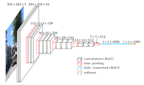
After AlexNet, the next innovation was VGG-Net, which came in two variants: VGG16 and VGG19. These networks had several improvements over AlexNet. First of all, this network was deeper than AlexNet. Work had been done just a year prior by Zeiler and Fergus that demonstrated deeper networks learned better. And, as we progress deeper into the network, the convolutional filters start to build on each other: the earlier layers are just line and edge detectors, but the later layers combine the earlier layers into shape and face detectors!

Source (https://www.cs.toronto.edu/~frossard/post/vgg16/)

Another improvement was that VGGNet used successive convolutional layers instead of the CONV – POOL architecture defined by LeNet. In the network, there are blocks of sequential convolutional layers, e.g., the CONV – CONV – CONV in the middle and end of the network. The danger of using successive convolutions at the time was that the network would become too large and training would take a long time to train. However, with new GPUs providing more computational power, this concern was quickly dismissed. This is the upwards trend on depth and computation that we’ll notice as we progress.

VGG-Net produced a smaller error than AlexNet in the ImageNet Large Scale Visual Recognition Challenge (ILSVRC) in 2014.

GoogLeNet

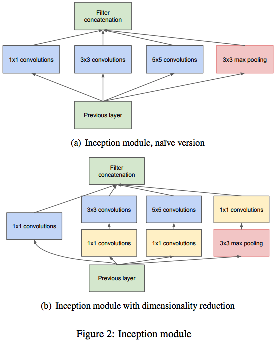
The network that won the ILSVRC in 2014 was GoogLeNet from Google, of course. The real novelty of this network is the Inception Modules. The network itself simply stacked these inception modules together.

Source (Going Deeper with Convolutions by Szegedy et al.)

The motivation behind these inception modules was around the issue of selecting the right filter or kernel size.We always prefer to use smaller filters, like 3×3 or 5×5 or 7×7, but which ones of theses works the best? Depending on how deep we make our network, each convolutional layer has a choice between 3 different filter sizes. If our network was $d$ layers deep, then we essentially have to try $3^d$ possible combinations, i.e., for each convolutional layer, we have 3 possible combinations so $3\cdot 3\cdot 3\dots 3$ $d$ times is $3^d$ .

Instead of doing this, the inception modules just accept that fact that choosing this is difficult: so why not choose all of them? Instead of choosing just a single filter size, choose all of them and concatenate the results. Taking the activation maps of features from the previous layer, we apply 3 separate convolutions and one pooling on top of that single input and concatenate the resulting feature maps together.

For example, if our input was $h_1\times w_1\times d_1$ and our output feature maps were $h_2\times w_2$ , then we can apply convolutions to our input to produce $h_2\times w_2\times \sum_i d^{(i)}$ where the sum is over all of the number of filters for all of the convolutional layers. We have to adjust the padding and spacing of our convolutions since the pooling layer will reduce the width and height of our input and the outputs must all have to same width and height to concatenate together.

There is one issue with this approach: computational complexity. An inception module is slow for high-dimensionality input. The solution is to convert that high-dimensionality input to a lower dimensionality using 1×1 convolutions. These kinds of convolutions are actually fully-connected layers!

For example, if our input was $64\times 64\times 128$ , applying a convolutional layer of 1×1 convolutions with 32 filters produces an output of $64\times 64\times 32$ (assuming no padding). This effectively reduced the dimension of our input! Those 32 1×1 filters are really just single neurons and their weights are learned just like everything else in the network!

The improved inception modules use these dimensionality-reducing 1×1 convolutions before applying the 3×3 and 5×5 convolutional layers. We also perform dimensionality reduction after the max pooling layer as well, for the same reason.

Now that we understand how an inception module works, we can apply them in GoogLeNet. As mentioned before, we simply stack many of these inception modules on top of each other to create GoogLeNet. (There are a few layers before we get to the stacks of inception module, and the graphic also shows auxiliary classifiers.)

Source (Going Deeper with Convolutions by Szegedy et al.)

This network was even deeper than the VGG19 network that also participated in the ILSVRC the same year. GoogLeNet won the image classification challenge in 2014, and won again in 2016 after they iterated on it (Inception v4).

ResNet

The network that won the 2015 ILSVRC is also the deepest network to this day: ResNet, or residual networks. The major issue with taking something like GoogLeNet and extending it many layers is the vanishing gradient problem.

With any network, we compute the error gradient at the end of the network and use backpropagation to propagate our error gradient backwards through the network. Using the chain rule, we have to keep multiplying terms with the error gradient as we go backwards. However, in the long chain of multiplication, if we multiply many things together that are less than 1, then the final result will be very small. This applies to the gradient as well: the gradient becomes very small as we approach the earlier layers in a deep architecture. This small gradient is an issue because then we can’t update the network parameters by a large enough amount and training is very slow. In some cases, the gradient actually becomes zero, meaning we don’t update the earlier parameters at all!

Whenever we backpropagate through an operation, we have to use the chain rule and multiply, but what if we were to backpropagate through the identity function? Then the gradient would simply be multiplied by 1 and nothing would happen to it! This is the idea behind ResNet: it stacks these residual blocks together where we use an identity function to preserve the gradient.

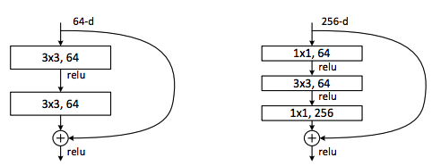
Source (Deep Residual Learning for Image Recognition by He et al.)

The beauty of residual blocks is the simplicity behind it. We take our input, apply some function to it and add it to our original input. Then, when we take the gradient, it is simply 1.

Mathematically, we can represent the residual block like this.

$H(x) = F(x) + x$

So when we find the partial derivative of the cost function $C$ with respect to $x$ , we get the following.

$\begin{align*} \displaystyle\frac{\partial C}{\partial x} &= \displaystyle\frac{\partial C}{\partial H} \displaystyle\frac{\partial H}{\partial x}\\ & = \displaystyle\frac{\partial C}{\partial H} (\displaystyle\frac{\partial F}{\partial x} + 1)\\ & = \displaystyle\frac{\partial C}{\partial H} \displaystyle\frac{\partial F}{\partial x} + \displaystyle\frac{\partial C}{\partial H} \end{align*}$

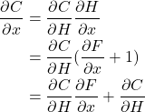
(A minor point: we can use a learned matrix in case $x$ and $F(x)$ are of a different dimensionality to make them compatible for addition.)

With that addition, the gradient is less likely to go to zero and we simply propagate the complete gradient backwards. These residual connections act as a “gradient highway” since the gradient distributes evenly at sums in a computation graph. This allows us to preserve the gradient as we go backwards.

Additionally, we can have bottleneck residual blocks, as shown on the right-side of the figure. We use those 1×1 convolutions again to reduce dimensionality before and after the middle convolutional layer.

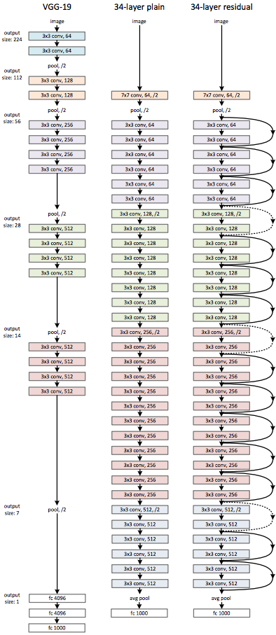
It turns out that these residual blocks are so powerful that we can stack many of these to produce networks that are over 5 times deeper than before! The deepest variant of ResNet was ResNet 151. That’s 151 layers deep! Before that, GoogLeNet was a mere 22 layers deep!

Source (Deep Residual Learning for Image Recognition by He et al.)

ResNets revolutionized deep architectures and now researchers are starting to use skip connections to make their architectures deeper. ResNets swept the ILSVRC in 2015!

DenseNet

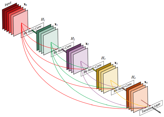
The most recent new architecture is from Facebook AI Research (FAIR) and won best paper at the most prestigious computer vision conference: Computer Vision and Pattern Recognition (CVPR) in 2017. Their architecture was titled DenseNet. Like GoogLeNet and ResNet before it, DenseNet introduced a new block called a Dense Block and stacked these blocks on top of each other, with some layers in between, to build a deep network.

Source (Densely Connected Convolutional Networks by Huang et al.)

These dense blocks take the concept of residual networks a step further and connect every layer to every other layer! In other words, for a dense block, we consider all dense block before it as input and we produce an output that we feed into all subsequent dense blocks. To make the layers compatible with each other, we apply convolutions and batch normalizations. The benefit of doing this is that we encourage feature reuse, resolve the vanishing gradient problem, and (counter-intuitively!) have fewer parameters overall!

Source (Densely Connected Convolutional Networks by Huang et al.)

As mentioned before, DenseNets won the Best Paper award at CVPR 2017 and achieved state-of-the-art performance on another image classification challenge: CIFAR-1000. Additionally, their work showed that DenseNets actually have fewer than half the number of parameters than ResNets and are comparable in performance on ImageNet.

To summarize, we discussed several different architectures that are being used today in convolutional neural networks for image classification. We discussed a few of the early deep learning architectures, such as AlexNet and VGG Net. Then, we discussed Google’s architecture that used the inception modules called GoogLeNet that won the ILSVRC in 2014. After that, we discussed the deepest network to date: ResNets. Using these residual connections, we can mitigate the vanishing gradient problem and stack these together to get networks that are over 100 layers deep! Finally, we discussed a very recent paper called DenseNet that exploited densely connections between their Dense Blocks.

New deep convolutional neural network architectures are being created each day and tested for efficiency against these. Keep up-to-date on these cutting-edge new architectures!

AlexNet

VGG-Net

GoogLeNet

ResNet

DenseNet

Continue Learning

File Download Link