One challenge of neural or deep architectures is that it is difficult to determine what exactly is going on in the machine learning algorithm that makes a classifier decide how to classify inputs. This is a huge problem in deep learning: we can get fantastic classification accuracies, but we don’t really know what criteria a classifier uses to make its classification decision. However, decision trees can present us with a graphical representation of how the classifier reaches its decision.
We’ll be discussing the CART (Classification and Regression Trees) framework, which creates decision trees. First, we’ll introduce the concept of decision trees, then we’ll discuss each component of the CART framework to better understand how decision trees are generated.
Download the full code here.
Did you come across any errors in this tutorial? Please let us know by completing this form and we’ll look into it! FINAL DAYS: Unlock coding courses in Unity, Godot, Unreal, Python and more.
Table of contents
Trees and Binary Trees
Before discussing decision trees, we should first get comfortable with trees, specifically binary trees. A tree is just a bunch of nodes connected through edges that satisfies one property: no loops!
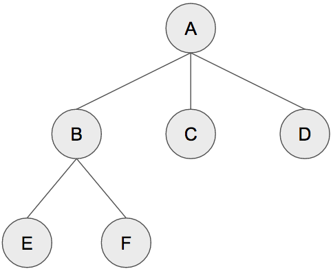
The above is an example of a tree. The nodes are A, B, C, D, E, and F. The edges are the lines that connect the nodes. The only rule we have to follow for this to be a valid tree is that it cannot have any loops or circuits.
Speaking of Node A, we consider it to be the root node, or our starting point, in other words. We conventionally pick the root node to be the node at the top of the tree. (Technically, any node in a tree can be the root). Node A has three children: Node B, Node C, and Node D. Child nodes are connected to the parent nodes through an edge. The only node without a parent is the root node. One other bit of terminology: Node E, Node F, Node C, and Node D are called leaf nodes because they are at the very bottom of the tree and have no children.
The depth of a tree is defined to be the number of levels, not including the root node. The tree above has a depth of 2 since Node B, Node C, and Node D are all on one level and Node E and Node F are on another level. In other words, it is the number of edges we have to traverse from the root to the farthest leaf node. Although Node A, the root, is on its own level, we usually do not include it when counting the depth of a tree. (If we have to consider it, we call it level 0.)
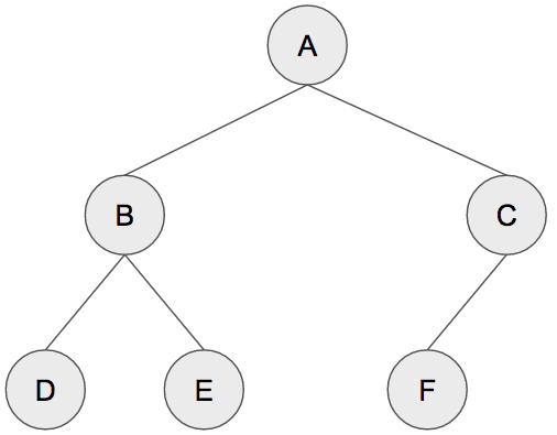
The tree above is a general tree, but it is not a binary tree. Decision trees are binary trees. Below is an example of a binary tree.
For a tree to be considered a binary tree, each parent node must have at most 2 child nodes. The above satisfies that condition. Parent nodes can have 0, 1, or 2 child nodes, but no greater than 2!
Decision Trees
Now that we have a basic understanding of binary trees, we can discuss decision trees. A decision tree is a kind of machine learning algorithm that can be used for classification or regression. We’ll be discussing it for classification, but it can certainly be used for regression. A decision tree classifies inputs by segmenting the input space into regions. Let’s consider the following data.
We can partition the 2D plane into regions where the points in each region belong to the same class. The splits or partitions are denoted with dashed lines: there’s one at ![]() ,
, ![]() , and
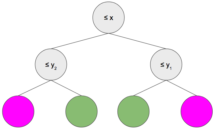
, and ![]() . This is an example segmentation that the decision tree might make. Under the hood, the decision tree represents this as a binary tree! Here’s the decision tree the corresponds to the above segmentation.
. This is an example segmentation that the decision tree might make. Under the hood, the decision tree represents this as a binary tree! Here’s the decision tree the corresponds to the above segmentation.
The structure, number of nodes, and positioning of the edges of our decision tree is not know a-priori but is built from our training data. We’ll soon discuss how we can create the tree from scratch using the CART framework. For now, let’s suppose that our decision tree is already created.
To classify a new input point, we simply traverse down the tree. At each node in the decision tree, we ask a question about our data point. For example, at the root node, we ask “is the x coordinate of our data point less than ![]() “? If it is, then we branch left. If it isn’t, we branch right. In general, if the condition at the node is met, we go left; if it is not true, then we go right. Suppose that the x coordinate of our node is indeed less than
“? If it is, then we branch left. If it isn’t, we branch right. In general, if the condition at the node is met, we go left; if it is not true, then we go right. Suppose that the x coordinate of our node is indeed less than ![]() , so we branch left. Now we ask “is the y coordinate of our node less than
, so we branch left. Now we ask “is the y coordinate of our node less than ![]() ? Let’s suppose that it isn’t. In this case, we go right and end up at a leaf node. The leaf nodes of a decision tree represent which class we assign to an input point. In our example, we know that our test point is in the green class. In our 2D plot, this particular test point is in the top-left region.
? Let’s suppose that it isn’t. In this case, we go right and end up at a leaf node. The leaf nodes of a decision tree represent which class we assign to an input point. In our example, we know that our test point is in the green class. In our 2D plot, this particular test point is in the top-left region.
There are some things to keep in mind about this demonstration of a decision tree. In our simple example, we alternated between considering the x coordinate and the y coordinate, but there’s no rule that says we have to do this. It is possible to have trees where we only consider a single dimension/feature for a few levels in the tree. Actually, decision trees work for data of any dimension, not just 2D data! Our simple example creates a segmentation where each region has 100% accuracy. While this is technically possible to do with a decision tree, it means we have overfit! We’ll discuss how to fix this when we talk about the CART framework.
Classification and Regression Trees (CART) Framework
Now that we have an intuitive understanding of how we use decision trees to classify points, let’s discuss how we build the tree in the first place! There are four points we have to consider:
- How many splits per node?
- Which dimension do we test?
- When do we stop?
- How do we assign class labels to the leaf nodes?
The first point is easy to address: we always use two splits at each node. Recall that a decision tree is a binary tree, so we need to make sure that there are no more than two splits per node.
But suppose we had several cases for a node, such as on the left. We have three regions: ![]() ,
, ![]() , and
, and ![]() .
.
We can still split it into two binary decisions, like on the right. First, split into ![]() and
and ![]() . Then we can split
. Then we can split ![]() into two regions:
into two regions: ![]() and
and ![]() . We can do this for any decision with any number of cases: split it into a sequence of binary decisions.
. We can do this for any decision with any number of cases: split it into a sequence of binary decisions.
But how do we even know which dimensions to check? Ideally, we want to choose values so that the resulting split causes one class to be much more present than the others. When we only have training data, at each node, we’ll be keeping track of how many examples of each class are present at a node as a vector ![]() where
where ![]() is the number of green examples and
is the number of green examples and ![]() is the number of magenta examples. We want to make splits so that we have many examples of only one particular class and few examples of the other.
is the number of magenta examples. We want to make splits so that we have many examples of only one particular class and few examples of the other.
In other words, we want the split that decreases the entropy. High entropy means that we have a mix of different classes; low entropy means that we have predominantly one class.
We want to make the split so that we decrease the entropy: the resulting split causes us to have many of one class and few of the other. Ideally, we want our nodes to have no entropy, i.e., all examples at this node are definitely of one class. This low entropy is desirable at the leaf nodes since, when we classify an example, we can be very sure of its class in a low entropy leaf node.
Mathematically, there are several ways to measure this. One way is using the definition of entropy.
![]()
This is computing the entropy at node ![]() by summing over all classes
by summing over all classes ![]() and computing
and computing ![]() where
where ![]() is the proportion of examples that belong to class
is the proportion of examples that belong to class ![]() at node
at node ![]() .
.
There is another, more commonly used metric called Gini impurity. Impurity and entropy mean the same thing: we want lower Gini impurity. We can compute the Gini impurity using the following.
![]()
We can check each one in order to make our split with categorical dimensions. This is trickier if we have continuous features. Specific algorithms use different techniques, such as considering only values that the features take or sampling along a dimension.
Now let’s address the third point: when do we stop splitting? Using a decision tree, we can keep splitting until each leaf node only has a single training example: that would be zero entropy/impurity! However, think of what this would look like graphically: we would have many small regions. In other words, we would overfit very much! On the other hand, we don’t want to stop splitting too early!
The solution to this is to fully build out the decision tree so that we overfit. Then, we can prune nodes, starting from the leaves. We compute the increase in entropy/impurity at the parent if we were to prune two child nodes, and perform the pruning if that entropy/impurity increase is below some constant or threshold. Varying this constant affects the depth of our decision tree: a small value won’t prune that much, but a large value will more aggressively prune the decision tree.
Finally, we have to address how we assign class labels to a leaf node. Ideally, at the leaf node, we’ll have zero entropy/impurity, and we simply select the only available class. However, in many cases, we won’t be that lucky. We might have a few examples from each class. There are several ways of handling this. A common thing to do is to randomly sample from the resulting distribution at that leaf node. We can also consider the total number of each class, i.e., we may have more green training examples than magenta, when assigning class labels.
Using the CART framework, we can build our human-readable decision tree!
Decision Tree Code
We’ll build and visualize a decision tree on the iris dataset. With scikit-learn, this is very easy to do!
from sklearn.datasets import load_iris
from sklearn import tree
from sklearn.metrics import classification_report, accuracy_score
from sklearn.model_selection import train_test_split
import graphviz

iris = load_iris()
X_train, X_test, y_train, y_test = train_test_split(iris.data, iris.target, test_size=0.4, random_state=17)

clf = tree.DecisionTreeClassifier(random_state=17)
clf = clf.fit(X_train, y_train)

y_pred = clf.predict(X_test)
print(classification_report(y_test, y_pred, target_names=iris.target_names))
print('\nAccuracy: {0:.4f}'.format(accuracy_score(y_test, y_pred)))
We load the iris dataset and split it into training and testing data. We can then construct a decision tree classifier and train! We evaluate on the test data and print the detailed precision, recall, and F1 score. We also compute the accuracy (around 95%).
To visualize the decision tree, we’ll need to install graphviz (brew install graphviz or sudo apt-get install graphviz ).
dot = tree.export_graphviz(clf, out_file=None, feature_names=iris.feature_names, class_names=iris.target_names, filled=True, rounded=True, special_characters=True)

graph = graphviz.Source(dot)
graph.format = 'png'
graph.render('iris', view=True)
We’re using the feature names of the dataset so that we don’t reference the dimension number (remember that the iris dataset has 4 features: petal width, petal length, sepal width, and sepal length).
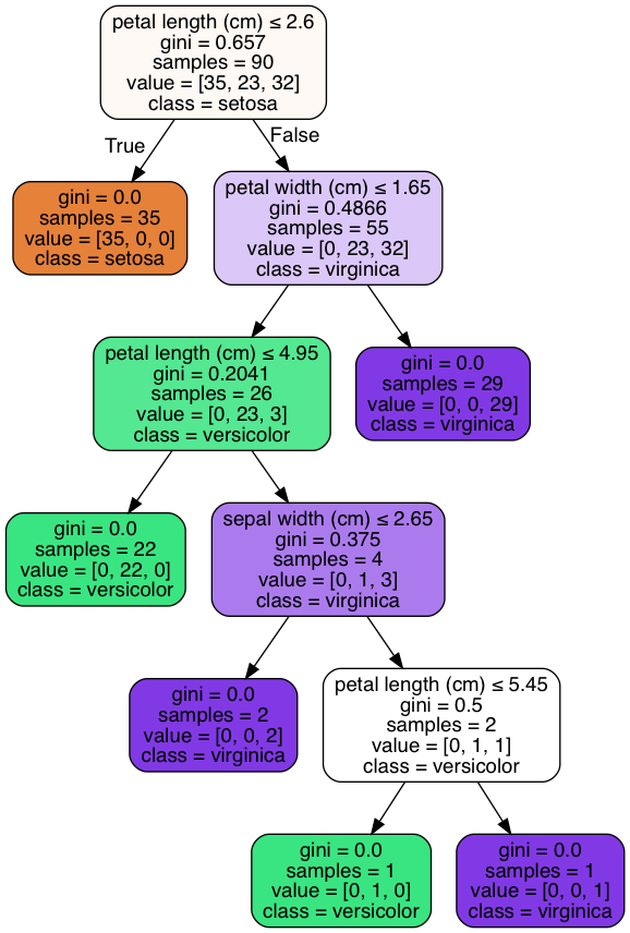
We should see the following image in the same directory as the Python file.
At each node, we ask a question about the features. If the answer to the question is yes, we go left, if not, we go right. Samples tells us how many examples are at that node, and the value is that vector of samples for each class. We’re using the Gini impurity as our metric, and notice how it is zero at each leaf node. Given test data, we can simply follow this tree to arrive at the class label!
Now let’s mess with the minimum entropy threshold parameter to see if we can prune this tree and how that affects the accuracy. Let’s set it to 0.1. This will tell our classifier that it’s okay to prune children such that the entropy/impurity at the parent after pruning is less than 0.1.
clf = tree.DecisionTreeClassifier(random_state=17, min_impurity_decrease=0.1)
When we do this, we get about the same accuracy, but our tree is much smaller!
If we set this parameter to be too large, then everything will collapse into a single node with a poor accuracy. Remember that the larger the value, the more aggressive pruning!
To summarize, we discussed how to use build and use decision trees. They give us a very human-friendly way of interpreting how they make classification decisions. We first discussed trees and binary trees, then built the intuition behind how to use decision trees. We discussed how to build a decision tree using the Classification and Regression Tree (CART) framework. Finally, we used a decision tree on the iris dataset.
Decision Trees are one of the few machine learning algorithms that produces a comprehensible understanding of how the algorithm makes decisions under the hood.
