Classification With Support Vector Machines

One of the most widely-used and robust classifiers is the support vector machine. Not only can it efficiently classify linear decision boundaries, but it can also classify non-linear boundaries and solve linearly inseparable problems. We’ll be discussing the inner workings of this classification jack-of-all-trades. We first have to review the perceptron so we can talk about support vector machines. Then we’ll derive the support vector machine problem for both linearly separable and inseparable problems. We’ll discuss the kernel trick, and, finally, we’ll see how varying parameters affects the decision boundary on the most popular classification dataset: the iris dataset.

Download the full code here.

Did you come across any errors in this tutorial? Please let us know by completing this form and we’ll look into it!

FREE COURSES

FINAL DAYS: Unlock coding courses in Unity, Godot, Unreal, Python and more.

ACCESS FOR FREE

Table of contents

Perceptron Review

Before continuing on to discuss support vector machines, let’s take a moment to recap the perceptron.

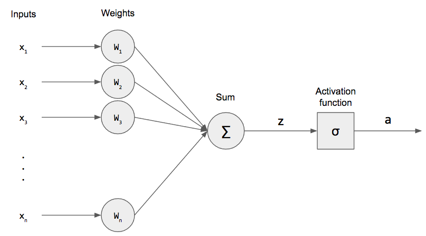
The perceptron takes a weighted sum of its inputs and applies an activation function. To train a perceptron, we adjust the weights of the weighted sum. The activation function can be any number of things, such as the sigmoid, hyperbolic tangent (tanh), or rectified linear unit (ReLU). After applying the activation function, we get an activation out, and that activation is compared to the actual output to measure how well our perceptron is doing. If it didn’t correctly classify our data, then we adjust the weights. We keep iterating over our training data until the perceptron can correctly classify each of our examples (or we hit the maximum number of epochs).

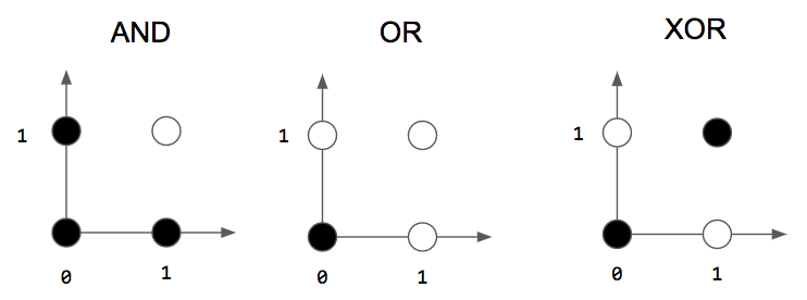
We trained our perceptron to solve logic gates but came to an important realization: the perceptron can only solve linear problems! In other words, the perceptron’s weights create a line (or hyperplane)! This is the reason we can’t use a single perceptron to solve the XOR problem.

Let’s discuss just linear problems for now. One of the most useful properties of the perceptron is the perceptron convergence theorem: for a linearly separable problem, the perceptron is guaranteed to find an answer in a finite amount of time.

However, there is one big catch: it finds the first line that correctly classifies all examples, not the best line. For any problem, if there is a single line that can correctly classify all training examples, there are an infinite number of lines that can separate the classes! These separating lines are also called decision boundaries because they determine the class based on which side of the boundary an example falls on.

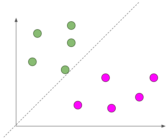
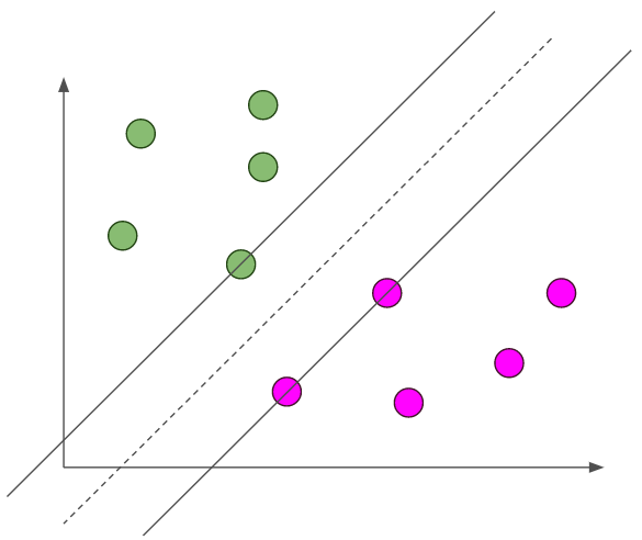
Let’s see an example to make this more concrete. Suppose we had the given data for a binary classification problem. If we used a perceptron, we might get a decision boundary that looks like this.

This isn’t the best decision boundary! The line is really close to all of our green examples and far from our magenta examples. If we get new examples, then we might have an example that’s really close to the decision boundary, but on the magenta side. If I didn’t draw that line, we would certainly think that the new point would be a green point. But, since it is on the other side of the decision boundary, even though it is closer to the green examples, our perceptron would classify it as a magenta point. This is not good!

If this decision boundary is bad, then where, among the infinite number of decision boundaries, is the best one? Our intuition tell us that the best decision boundary should probably be oriented in the exact middle of the two classes of data.

The dashed line is the decision boundary. This seems like a better fit! Now, if we have a new example that’s really close to this decision boundary, we still can classify it correctly! But how do we find this best decision boundary?

Support Vector Machines

The goal of support vector machines (SVMs) is to find the optimal line (or hyperplane) that maximally separates the two classes! (SVMs are used for binary classification, but can be extended to support multi-class classification). Mathematically, we can write the equation of that decision boundary as a line.

$g(\mathbf{x}) = \mathbf{w}^T \mathbf{x} + b = 0$

Note that we set this equal to zero because it is an equation. Depending on the value of $g$ for a particular point $\mathbf{x}$ , we can classify into the two classes. We’re using vector notation to be as general as possible, but this works for a simple 2D (one input) case as well.

If we do some geometry, we can figure out that the distance from any point to the decision boundary is the following

$r = \displaystyle\frac{g(\mathbf{x})}{||\mathbf{w}||}$

Our goal is to maximize $r$ for the points closest to the optimal decision boundary. These points are so important that they have a special name: support vectors!

We can actually simplify this goal a little bit by considering only the support vectors. Notice that the numerator just tells us which class (we’re assuming the two classes are 1 and -1), but the denominator doesn’t change. We can take the absolute value of each side to get rid of the numerator.

$|r| = \displaystyle\frac{1}{||\mathbf{w}||}$

where $\mathbf{w}$ is the optimal decision boundary (later we’ll show that the bias is easy to solve for if we know $\mathbf{w}$ ) We can simplify even further! Maximizing $\frac{1}{||\mathbf{w}||}$ is equivalent to minimizing $||\mathbf{w}||$ . This is a bit tricky to do mathematically, so we can just square this to get $\min \frac{1}{2}\mathbf{w}^T\mathbf{w}$ . (The constant out front is there so it can nicely cancel out later!)

However, we need more constraints, else we could just make $||\mathbf{w}||=0$ ! That wouldn’t solve anything! The other constraints come from our need to correctly classify the examples!

$y_i (\mathbf{w}^T\mathbf{x}_i + b) \geq 1~~~~\forall i$

where $y_i$ is the ground truth and we iterate over our training set. To see why this is correct, let’s split it into the two classes 1 and -1:

$\begin{align*} \mathbf{w}^T\mathbf{x}_i + b &\geq 1~~~~~~\forall y_i = 1\\ \mathbf{w}^T\mathbf{x}_i + b &\leq -1 ~~~~\forall y_i = -1 \end{align*}$

We can compress the two into the single equation above. After we’ve considered all of this, we can formally state our optimization problem! (In the constraints, the 1 was moved over to the other side of the inequality.)

$\begin{align*} & \text{minimize} & & \frac{1}{2}\mathbf{w}^T\mathbf{w} \\ & \text{subject to} & & y_i (\mathbf{w}^T\mathbf{x}_i + b) -1 \geq 0~~~~\forall i \end{align*}$

This is called the primal problem. This is a run-of-the-mill optimization problem, so we can use the technique of Lagrange Multipliers to solve this problem.

$\mathcal{L} = \displaystyle\frac{1}{2}\mathbf{w}^T\mathbf{w} - \displaystyle\sum_{i=1}^N \alpha_i [y_i (\mathbf{w}^T\mathbf{x}_i + b) - 1 ]$

where the $\alpha_i$ ‘s are the Lagrange multipliers. To solve this, we have to compute the partial derivatives with respect to our weights and bias, set them to zero, and solve! I’ll skip over the derivation and just give the solutions.

$\begin{align*} \mathbf{w} &= \displaystyle\sum_{i=1}^N \alpha_i y_i\mathbf{x}_i\\ \displaystyle\sum_{i=1}^N \alpha_i y_i &= 0 \end{align*}$

The first equation is $\frac{\partial\mathcal{L}}{\partial\mathbf{w}}$ and the second equation is $\frac{\partial\mathcal{L}}{\partial b}$ . These solutions tell us some useful things about the weights and Lagrange multipliers. In particular, they give some constraints on the Lagrange multipliers. These $\alpha_i$ ‘s also tell us something very important about our SVM: they indicate the support vectors! If a particular point $\mathbf{x}_i$ is a support vector, then its corresponding Lagrange multiplier $\alpha_i$ will be greater than 0! If it is not a support vector, then it will be equal to 0!

However, we still don’t have enough information to solve our problem. As it turns out, there is a corresponding problem called the dual problem that we can solve instead.

$\begin{align*} & \text{maximize} & & \displaystyle\sum_{i=1}^N \alpha_i - \displaystyle\frac{1}{2} \displaystyle\sum_{i=1}^N \displaystyle\sum_{j=1}^N \alpha_i \alpha_j y_i y_j \mathbf{x}_i^T \mathbf{x}_j \\ & \text{subject to} & & \displaystyle\sum_{i=1}^N \alpha_i y_i = 0~~~~\forall i\\ &&& \alpha_i \geq 0~~~~\forall i \end{align*}$

This is something that we can solve! Notice that it’s only in terms of the Lagrange multipliers! Everything else is known! We usually use a quadratic programming solver to do this for us because it is infeasible to solve by-hand for large numbers of points. But we would solve for this by setting each $\frac{\partial\mathcal{L}}{\partial\alpha_i} = 0$ and solving.

After we’ve solved for the $\alpha_i$ ‘s, we can find the optimal line using the following equations.

$\begin{align*} \mathbf{w} &= \displaystyle\sum_{i=1}^N \alpha_i y_i\mathbf{x}_i\\ b &= \underset{i\in N}{\text{average}} \frac{1}{y_i} - \mathbf{w}^T\mathbf{x}_i \end{align*}$

The first is from the primal problem, and the second is just solving for the bias from the decision boundary equation.

SVMs for Logic Gates

Let’s take a break from the math and apply support vector machines to a simple logic gate, like what we did for perceptrons. In particular, let’s train an SVM to solve the logic AND gate.

import numpy as np
import matplotlib.pyplot as plt
from sklearn import svm, datasets

X = np.array([
    [0, 0],
    [0, 1],
    [1, 0],
    [1, 1]
])
y = np.array([0, 0, 0, 1])

clf = clf.SVC(kernel='linear', C=1e6)
clf.fit(X, y)

We’re building a linear decision boundary. Ignore the other parameter $C$ ; we’ll discuss that later. Now we can use some plotting code (source) to show the decision boundary and support vectors.

plt.scatter(X[:, 0], X[:, 1], c=y, s=30, cmap=plt.cm.Paired)

# plot the decision function
ax = plt.gca()
xlim = ax.get_xlim()
ylim = ax.get_ylim()

# create grid to evaluate model
xx = np.linspace(xlim[0], xlim[1], 30)
yy = np.linspace(ylim[0], ylim[1], 30)
YY, XX = np.meshgrid(yy, xx)
xy = np.vstack([XX.ravel(), YY.ravel()]).T
Z = clf.decision_function(xy).reshape(XX.shape)

# plot decision boundary and margins
ax.contour(XX, YY, Z, colors='k', levels=[-1, 0, 1], alpha=0.5, linestyles=['--', '-', '--'])
# plot support vectors
ax.scatter(clf.support_vectors_[:, 0], clf.support_vectors_[:, 1], s=100, linewidth=1, facecolors='none')
plt.show()

Before we plot this, let’s try to predict what our decision boundary and surface will look like. Here’s the picture of the logic gates again.

Where will the decision boundary be? Which points will be the support vectors? The decision boundary will be a diagonal line between the two classes. The support vectors will be (1,1), (0,1), and (1,0) since they are closest to that boundary.

This matches our intuition! So SVMs can certainly solve linear separable problems, but what about non-linearly separable problems?

SVMs for Linearly Inseparable Problems

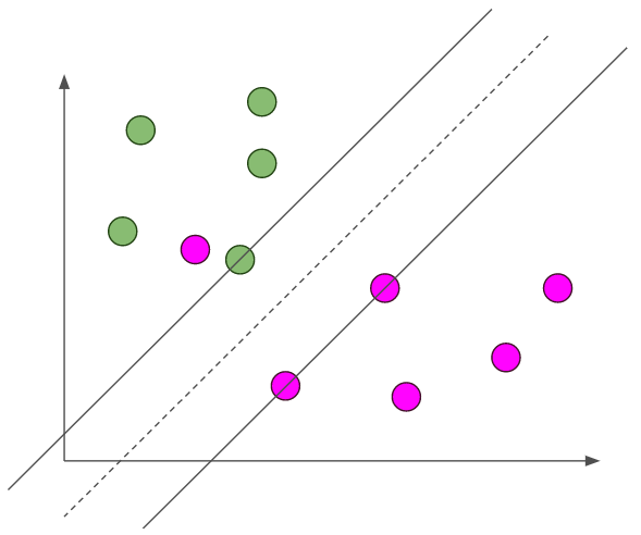
Suppose we had the following linearly inseparable data.

There is no line that can correctly classify each point! Can we still use our SVM? We can, but with a modification. We have to add slack variables $xi_i$ . These measure how many misclassifications there are. We also want to minimize the sum of all of the slack variables. Intuitively, this corresponds to minimizing the number of incorrect classifications. We can reformulate our primal problem.

$\begin{align*} & \text{minimize} & & \frac{1}{2}\mathbf{w}^T\mathbf{w} + C\displaystyle\sum_{i=0}^N \xi_i \\ & \text{subject to} & & y_i (\mathbf{w}^T\mathbf{x}_i + b) - 1 + \xi_i \geq 0~~~~\forall i\\ &&& \xi_i \geq 0~~~~\forall i \end{align*}$

where we introduce a new hyperparameter $C$ that measures the tradeoff between the two objectives: largest margin of separation and smallest number of incorrect classifications. And, from there, go to our corresponding dual problem.

This looks almost the same as before! The change is that our $\alpha_i$ ‘s are also bounded above by $C$ . After solving for our $\alpha_i$ ‘s, we can solve for our weights and bias exactly the same as in our linearly separable case!

The Kernel Trick

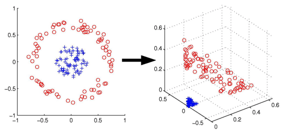
One last topic to discuss is the kernel trick. Instead of having a linear decision boundary, we can have a nonlinear decision boundary. The idea behind the kernel trick is to apply a nonlinear kernel to our inputs $\mathbf{x}_i$ to transform them into a higher-dimensional space where we can find a linear decision boundary.

Consider the above figure. The left is our 2D dataset that can’t be separated using a line. However, if we use some kernel function $\varphi(\mathbf{x}_i)$ to project all of our points into a 3D space, then we can find a plane that separates our examples. The intuition behind this is that higher dimensional spaces have extra degrees of freedom that we can use to find a linear plane! There are many different choices of kernel functions: radial basis functions, polynomial functions, and others.

SVM for The Iris Dataset

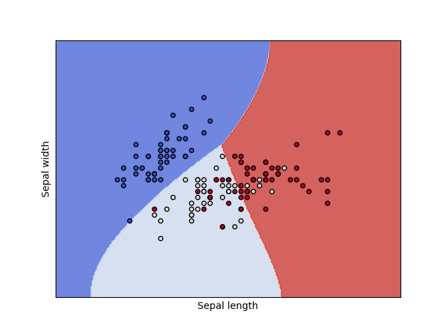
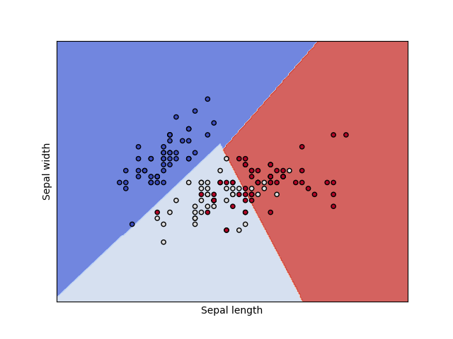
One of the most famous datasets in all of machine learning is the iris dataset. It has 150 data points across 3 different types of flowers. The features that were collected were sepal length/width and petal length/width. Our goal is to use an SVM to correctly classify an input into the correct flower and to draw the decision boundary.

Since the iris dataset has 4 features, let’s consider only the first two features so we can plot our decision regions on a 2D plane. First, let’s load the iris dataset, create our training and testing data, and fit our SVM. We’ll change some parameters later, but let’s use a linear SVM.

iris = datasets.load_iris()
X = iris.data[:, :2]
y = iris.target

C = 1.0 
clf = svm.SVC(kernel='linear', C=C)
clf.fit(X, y)

Now we can use some auxiliary functions (source) to plot our decision regions.

ax = plt.gca()
def make_meshgrid(x, y, h=.02):
    x_min, x_max = x.min() - 1, x.max() + 1
    y_min, y_max = y.min() - 1, y.max() + 1
    xx, yy = np.meshgrid(np.arange(x_min, x_max, h), np.arange(y_min, y_max, h))
    return xx, yy


def plot_contours(ax, clf, xx, yy, **params):
    Z = clf.predict(np.c_[xx.ravel(), yy.ravel()])
    Z = Z.reshape(xx.shape)
    out = ax.contourf(xx, yy, Z, **params)
    return out

plot_contours(ax, clf, xx, yy, cmap=plt.cm.coolwarm, alpha=0.8)
ax.scatter(X0, X1, c=y, cmap=plt.cm.coolwarm, s=20, edgecolors='k')
ax.set_xlim(xx.min(), xx.max())
ax.set_ylim(yy.min(), yy.max())
ax.set_xlabel('Sepal length')
ax.set_ylabel('Sepal width')
ax.set_xticks(())
ax.set_yticks(())

plt.show()

Additionally, we’re going to print the classification report to see how well our SVM performed.

from sklearn.metrics import classification_report
print(classification_report(y, clf.predict(X), target_names=iris.target_names))

Now let’s run our code to see a plot and classification metrics!

Additionally, we can try using an RBF kernel and changing our $C$ value. Recall that $C$ controls the tradeoff between large margin of separation and a lower incorrect classification rate.

C = 1.0 
clf = svm.SVC(kernel='rbf', C=C)

Try varying different parameters to get the best classification score – and feel free to add all this to your own coding portfolio as well!

To summarize, Support Vector Machines are very powerful classification models that aim to find a maximal margin of separation between classes. We saw how to formulate SVMs using the primal/dual problems and Lagrange multipliers. We also saw how to account for incorrect classifications and incorporate that into the primal/dual problems. Finally, we trained an SVM on the iris dataset.

Support Vector Machines are one of the most flexible non-neural models for classification; they’re able to model linear and nonlinear decision boundaries for linearly separable and inseparable problems.