All About Autoencoders

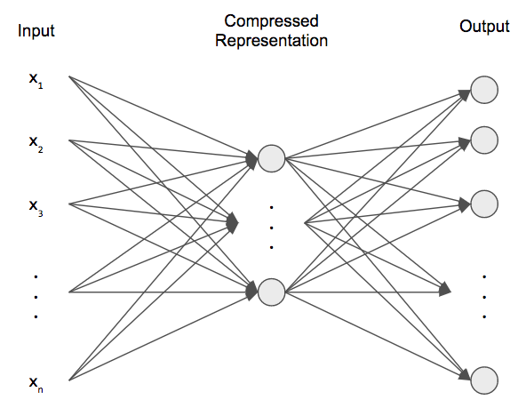
Data compression is a big topic that’s used in computer vision, computer networks, computer architecture, and many other fields. The point of data compression is to convert our input into a smaller representation that we recreate, to a degree of quality. This smaller representation is what would be passed around, and, when anyone needed the original, they would reconstruct it from the smaller representation.

Consider a ZIP file. When we create a ZIP file, we compress our files so that they take up fewer bytes. Then we pass around that ZIP file. If we wanted to access the contents, we can uncompress the ZIP file, and reconstruct the contents from the ZIP file.

In another example, consider a JPEG image file. This is an example of a lossy format: when we compress a JPEG, we lose information about the original. If we uncompress it, then our reconstruction isn’t perfect. However, for JPEG, we can compress it down to a tenth of the original data without any noticeable loss in image quality!

Many techniques in the past have been hard-coded or use clever algorithms. Autoencoders are unsupervised neural networks that use machine learning to do this compression for us. There are many different kinds of autoencoders that we’re going to look at: vanilla autoencoders, deep autoencoders, deep autoencoders for vision. Finally, we’ll apply autoencoders for removing noise from images.

Download the full code here.

Did you come across any errors in this tutorial? Please let us know by completing this form and we’ll look into it!

FREE COURSES

FINAL DAYS: Unlock coding courses in Unity, Godot, Unreal, Python and more.

ACCESS FOR FREE

Vanilla Autoencoder

We’ll first discuss the simplest of autoencoders: the standard, run-of-the-mill autoencoder. Essentially, an autoencoder is a 2-layer neural network that satisfies the following conditions.

1. The hidden layer is smaller than the size of the input and output layer.
2. The input layer and output layer are the same size.

The hidden layer is compressed representation, and we learn two sets of weights (and biases) that encode our input data into the compressed representation and decode our compressed representation back into input space.

Notice that there are no labels! Our input and output are the same! But then what is our loss function? We have a simple Euclidean distance loss: called the reconstruction error, where the input is and the reconstruction is . We want to minimize this error. In other words, this error represents how close our reconstruction was to the true input data. We won’t expect a perfect reconstruction since the number of hidden neurons is less than the number of input neurons, but we want the parameters to give us the best possible reconstruction.

Mathematically, our above autoencoder can be thought of as two separate things: an encoder and decoder.

where the superscripts correspond to the encoder and decoder and the input is . Hence, our loss function will be the squared Euclidean error.

When we train our autoencoder, we’re trying to minimize . We won’t see the backpropagation derivation of the update rules, but they’re identical to a standard neural network.

The big catch with autoencoders is that they only work for the data we train them on! If we train our autoencoder on images of cats, then it won’t work too well for images of dogs!

This is all there is to autoencoders! They’re simple neural networks but also very powerful! Let’s code up an autoencoder.

First, we’ll need to load our MNIST handwritten digits dataset. Notice that we’re not loading any of the labels because autoencoders are unsupervised. Additionally, we rescale our images from 0 – 255 to 0 – 1 and flatten them out.

from keras.layers import Input, Dense
from keras.models import Model
from keras.datasets import mnist

import numpy as np
import matplotlib.pyplot as plt

(X_train, _), (X_test, _) = mnist.load_data()
X_train = X_train.astype('float32') / 255.
X_test = X_test.astype('float32') / 255.
X_train = X_train.reshape((X_train.shape[0], -1))
X_test = X_test.reshape((X_test.shape[0], -1))

A numpy trick to flatten the rest of the dimension is to use -1 to infer the new dimension’s size based on the old one. Since our input is 60000x28x28, using -1 for the last dimension, will effectively flatten the rest of the dimensions. Hence, our resulting shape is 60000×784, for the training data.

Now we can create our autoencoder! We’ll use ReLU neurons everywhere and create constants for our input size and our encoding size. Notice that our hidden layer size is much smaller than our input!

INPUT_SIZE = 784
ENCODING_SIZE = 64

input_img = Input(shape=(INPUT_SIZE,))
encoded = Dense(ENCODING_SIZE, activation='relu')(input_img)
decoded = Dense(INPUT_SIZE, activation='relu')(encoded)
autoencoder = Model(input_img, decoded)

Now we simply build and train our model. We’ll use the ADAM optimizer and mean squared error loss (the Euclidean distance/loss) between the input and reconstruction.

autoencoder.compile(optimizer='adam', loss='mean_squared_error')
autoencoder.fit(X_train, X_train, epochs=50, batch_size=256, shuffle=True, validation_split=0.2)

After our autoencoder has trained, we can try to encode and decode the test set to see how well our autoencoder can compress.

decoded_imgs = autoencoder.predict(X_test)

Finally, we can visualize our true values and reconstructions using matplotlib.

plt.figure(figsize=(20, 4))
for i in range(10):
    # original
    plt.subplot(2, 10, i + 1)
    plt.imshow(X_test[i].reshape(28, 28))
    plt.gray()
    plt.axis('off')

    # reconstruction
    plt.subplot(2, 10, i + 1 + 10)
    plt.imshow(decoded_imgs[i].reshape(28, 28))
    plt.gray()
    plt.axis('off')

plt.tight_layout()
plt.show()

We can see the results below. The top row is the input and the bottom row is the reconstruction.

That’s not a bad reconstruction! By training only 50 epochs, we get decent reconstructions! If we wanted to be more rigorous about it, we could plot the loss functions of training and validation to ensure we had a low reconstruction loss, but, qualitatively, these look great!

Deep Autoencoders

We can apply the deep learning principle and use more hidden layers in our autoencoder to reduce and reconstruct our input. Our hidden layers have a symmetry where we keep reducing the dimensionality at each layer (the encoder) until we get to the encoding size, then, we expand back up, symmetrically, to the output size (the decoder).

Let’s take a look at how we can modify our autoencoder to be a deep autoencoder. Making this change is fairly simple.

input_img = Input(shape=(INPUT_SIZE,))
encoded = Dense(512, activation='relu')(input_img)
encoded = Dense(256, activation='relu')(encoded)
encoded = Dense(128, activation='relu')(encoded)

encoded = Dense(ENCODING_SIZE, activation='relu')(encoded)

decoded = Dense(128, activation='relu')(encoded)
decoded = Dense(256, activation='relu')(decoded)
decoded = Dense(512, activation='relu')(decoded)
decoded = Dense(INPUT_SIZE, activation='relu')(decoded)
autoencoder = Model(input_img, decoded)

We reduce our input from 784 -> 512 -> 256 -> 128 -> 64, then expand it back up 64 -> 128 -> 256 -> 512 -> 784. The rest of the code is exactly the same.

These reconstructions look a bit better! If we plotted and compared the losses, this deeper autoencoder model actually has a smaller loss value than the shallow autoencoder model.

Convolutional Autoencoder

Remember that the MNIST data is image data. When we flatten it, we’re not making full use of the spatial positioning of the pixels in the image. This is the same problem that plagued artificial neural networks when they were trying to work with image data. Instead, we developed Convolutional Neural Networks to handle image data.

(If you are not familiar with convolutional neural networks, please read the post here.)

Similarly, we can use convolutional autoencoders! Instead of using fully-connected layers, we use convolutional and pooling layers to reduce our input down to an encoded representation. But then we have to somehow upscale our encoded representation back up to the same shape as the encoding. How do we do that?

The opposite of convolution is (misleadingly named) deconvolution, but, in reality, this is just applying plain, old convolution! So to “undo” a convolution, we simply apply another convolution! I won’t go into the details, but “undo-ing” a convolution corresponds to applying a transpose of a kernel, which is just convolution with a transposed kernel, which is just convolution! (A more apt name for deconvolution is convolution transposed.)

The opposite of pooling is upsampling. This works in the exact same way as pooling, but in reverse. For pooling, we split the image up into non-overlapping regions of a particular size and take the max of each region to become the new pixel (for max pooling). For example, if we had a pooling layer with a 2×2 window size, then each 2×2 window in the input corresponds to a single pixel in the output. For upsampling, we reverse this. For each pixel in the input, we expand it out to encompass a window. If we had a 2×2 upsampling window, then each pixel in the input is resized to a 2×2 region. There are fancier ways we can do this, e.g., fancy interpolation, but upsampling works well in practice.

When coding a convolutional autoencoder, we have to make sure our input has the correct shape. The MNIST data we get will be only 28×28, but we also expect a dimension that tells us the number of channels. MNIST is in black-and-white, so we only have a single channel. We can easily extend our data by a dimension using numpy’s newaxis. The ellipsis before the newaxis just means to leave everything else as is. This effectively changes our shape from 28×28 to 28x28x1 (and the batch size is included as the first dimension).

from keras.layers import Input, Dense, Conv2D, MaxPooling2D, UpSampling2D
from keras.models import Sequential
from keras.datasets import mnist

import numpy as np
import matplotlib.pyplot as plt

(X_train, _), (X_test, _) = mnist.load_data()
X_train = X_train.astype('float32') / 255.
X_test = X_test.astype('float32') / 255.
X_train = X_train[..., np.newaxis]
X_test = X_test[..., np.newaxis]

Now we can build our convolutional autoencoder! Notice that we’re using a slightly different syntax. Instead of using Keras’ functional notation, we’re using a sequential model where we simply add layers to it in the order we want. The functional syntax is for more advanced models where we might several inputs and several output or other non-sequential models. We could have represented the previous deep and shallow autoencoders with sequential models as well.

autoencoder = Sequential()
autoencoder.add(Conv2D(32, (3, 3), activation='relu', padding='same', input_shape=(28, 28, 1)))
autoencoder.add(MaxPooling2D((2, 2), padding='same'))
autoencoder.add(Conv2D(8, (3, 3), activation='relu', padding='same'))
autoencoder.add(MaxPooling2D((2, 2), padding='same'))
autoencoder.add(Conv2D(8, (3, 3), activation='relu', padding='same'))

# our encoding
autoencoder.add(MaxPooling2D((2, 2), padding='same'))

autoencoder.add(Conv2D(8, (3, 3), activation='relu', padding='same'))
autoencoder.add(UpSampling2D((2, 2)))
autoencoder.add(Conv2D(8, (3, 3), activation='relu', padding='same'))
autoencoder.add(UpSampling2D((2, 2)))
autoencoder.add(Conv2D(32, (3, 3), activation='relu'))
autoencoder.add(UpSampling2D((2, 2)))
autoencoder.add(Conv2D(1, (3, 3), activation='relu', padding='same'))

For each convolutional layer, we have a corresponding “deconvolutional” layer when we decode. For each max pooling layer, we have a corresponding upsampling layer. After we’ve constructed this architecture, we can simply build and fit our model.

autoencoder.compile(optimizer='adam', loss='mean_squared_error')
autoencoder.fit(X_train, X_train, epochs=50, batch_size=256, shuffle=True, validation_split=0.2)

Let’s take a look at the results of the convolutional autoencoder.

These results are much smoother! Notice that we’ve filled in some of the holes/gaps in our numbers. Just like how convolutional neural networks performed better than plain artificial neural networks on image tasks, convolutional autoencoders work better than plain autoencoders.

Denoising Autoencoder

One application of convolutional autoencoders is denoising. Suppose we have an input image with some noise. These kinds of noisy images are actually quite common in real-world scenarios. For a denoising autoencoder, the model that we use is identical to the convolutional autoencoder. However, our training and testing data are different. For our training data, we add random, Gaussian noise, and our test data is the original, clean image. This trains our denoising autoencoder to produce clean images given noisy images.

We’ll have to add noise to our training data. This is simple enough with numpy. We also have to clip our image pixels to .

(X_train, _), (X_test, _) = mnist.load_data()
X_train = X_train.astype('float32') / 255.
X_test = X_test.astype('float32') / 255.
X_train = X_train[..., np.newaxis]
X_test = X_test[..., np.newaxis]

X_train_noisy = X_train + 0.25 * np.random.normal(size=X_train.shape)
X_test_noisy = X_test + 0.25 * np.random.normal(size=X_test.shape)

X_train_noisy = np.clip(X_train_noisy, 0., 1.)
X_test_noisy = np.clip(X_test_noisy, 0., 1.)

We have to make some modifications to how we use our new, noisy data. When we fit our model, the input is the noisy data and the output is the clean data. Everything else is the same as the convolutional autoencoder.

autoencoder.fit(X_train_noisy, X_train, epochs=50, batch_size=256, shuffle=True, validation_split=0.2)

Now, we can plot the the noisy test examples and the denoised examples.

decoded_imgs = autoencoder.predict(X_test_noisy)

plt.figure(figsize=(20, 4))
for i in range(10):
    # original
    plt.subplot(2, 10, i + 1)
    plt.imshow(X_test_noisy[i].reshape(28, 28))
    plt.gray()
    plt.axis('off')

    # reconstruction
    plt.subplot(2, 10, i + 1 + 10)
    plt.imshow(decoded_imgs[i].reshape(28, 28))
    plt.gray()
    plt.axis('off')

plt.tight_layout()
plt.show()

Let’s see if our denoising autoencoder works.

We’ve successfully cleaned up our images! Given new images, we can apply our autoencoder to remove noise from our images. Remember that autoencoders are only as good as the data we train them on. Since we trained our autoencoder on MNIST data, it’ll only work for MNIST-like data!

To summarize, an autoencoder is an unsupervised neural network comprised of an encoder and decoder that can be used to compress the input data into a smaller representation and uncompress it. They don’t have to be 2-layer networks; we can have deep autoencoders where we symmetrically stack the encoder and decoder layers. Additionally, when dealing with images, autoencoders don’t have to use just fully-connected layers! We can use convolution and pooling, and their counterparts, to encode and decode image data! In fact, we noticed that we actually get better-looking reconstructions. One application of these convolutional autoencoders that we discussed was for image denoising. We can train an autoencoder to clean up noisy images and found they worked quite well!

Autoencoders are one of the simplest unsupervised neural networks that have a wide variety of use in compression.