Recurrent Neural Networks For Language Modeling

Many neural network models, such as plain artificial neural networks or convolutional neural networks, perform really well on a wide range of data sets. They’re being used in mathematics, physics, medicine, biology, zoology, finance, and many other fields. However, there is one major flaw: they require fixed-size inputs! The inputs to a plain neural network or convolutional neural network have to be the same size for training, testing, and deployment! This means we can’t use these architectures for sequences or time-series data.

But along comes recurrent neural networks to save the day! We’ll define and formulate recurrent neural networks (RNNs). We’ll discuss how we can use them for sequence modeling as well as sequence generation. Then we’ll code up a generic, character-based recurrent neural network from scratch, without any external libraries besides numpy! Finally, we’ll train our RNN on Shakespeare and have it generate new Shakespearean text!

Download the full code here.

Did you come across any errors in this tutorial? Please let us know by completing this form and we’ll look into it!

FREE COURSES

FINAL DAYS: Unlock coding courses in Unity, Godot, Unreal, Python and more.

ACCESS FOR FREE

Table of contents

Recurrent Neural Networks Formulation

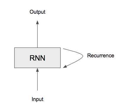
As we mentioned before, recurrent neural networks can be used for modeling variable-length data. The most general and fundamental RNN is shown above. The most important facet of the RNN is the recurrence! By having a loop on the internal state, also called the hidden state, we can keep looping for as long as there are inputs.

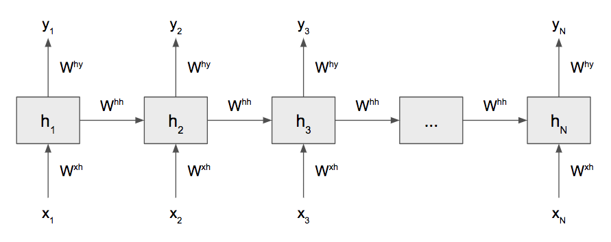
The above image can be a bit difficult to understand in practice, so we commonly “unroll” the RNN where we have a box for each time step, or input in the sequence.

For a particular cell, we feed in an input $\mathbf{x}_t$ at some time $t$ to get a hidden state $\mathbf{h}_t$ ; then, we use that to produce an output $\mathbf{y}_t$ . We keep doing this until we reach the end of the sequence. The most important part of an RNN is the recurrence, and that is modeled by the arrow that goes from one hidden state block to another. This recurrence indicates a dependence on all the information prior to a particular time $t$ . In other words, inputs later in the sequence should depend on inputs that are earlier in the sequence; the sequence isn’t independent at each time step!

For example, suppose we were doing language modeling. We have an input sentence: “the cat sat on the ____.” By knowing all of the words before the blank, we have an idea of what the blank should or should not be! This is the reason RNNs are used mostly for language modeling: they represent the sequential nature of language!

For our purposes, we’re going to be coding a character-based RNN. This takes character input and produces character output. We take our text and split it into individual characters and feed that in as input. However, we can’t directly feed text into our RNN. All neural networks work with numbers, not characters! However, we can easily convert characters to their numerical counterparts. We simply assign a number to each unique character that appears in our text; then we can convert each character to that number and have numerical inputs! Similarly, our output will also be numerical, and we can use the inverse of that assignment to convert the numbers back into texts.

(In practice, when dealing with words, we use word embeddings, which convert each string word into a dense vector. Usually, these are trained jointly with our network, but there are many different pre-trained word embedding that we can use off-the-shelf (Richard Socher’s pre-trained GloVe embeddings, for example). )

Like any neural network, we have a set of weights that we want to solve for using gradient descent: $\mathbf{W}^{(xh)}$ , $\mathbf{W}^{(hh)}$ , $\mathbf{W}^{(hy)}$ (I’m excluding the biases for now). Unlike other neural networks, these weights are shared for each time step! We use the same weights for each time step! This is also part of the recurrence aspect of our RNN: the weights are affected by the entire sequence. This makes training them a bit tricky, as we’ll discuss soon.

The above figure models an RNN as producing an output at each time step; however, this need not be the case. We can vary how many inputs and outputs we have, as well as when we produce those outputs.

(Credit: http://karpathy.github.io/2015/05/21/rnn-effectiveness/)

We can have several different flavors of RNNs:

One-to-one: the simplest RNN
One-to-many: sequence generation tasks
Many-to-one: sentiment analysis
Many-to-many: machine translation

Additionally, we can have bidirectional RNNs that feed in the input sequence in both directions! We can also stack these RNNs in layers to make deep RNNs. RNNs are just the basic, fundamental model for sequences, and we can always build upon them.

Backpropagation Through Time

Now that we understand the intuition behind an RNN, let’s formalize the network and think about how we can train it. For our purposes, we’re just going to consider a very simple RNN, although there are more complicated models, such as the long short-term memory (LSTM) cell and gated recurrent unit (GRU).

An RNN is essentially governed by 2 equations.

(1) $\begin{align*} \mathbf{h}_t &= \sigma(\mathbf{W}^{(xh)}\mathbf{x}_t + \mathbf{W}^{(hh)}\mathbf{h}_{t-1} + \mathbf{b}^{(h)})\\ \mathbf{y}_t &= \mathbf{W}^{(hy)}\mathbf{h}_{t} + \mathbf{b}^{(y)} \end{align*}$

The first defines the recurrence relation: the hidden state at time $t$ is a function of the input at time $t$ and the previous hidden state at time $t-1$ . For $\mathbf{h}_0$ , we usually initialize that to the zero vector. For our nonlinearity, we usually choose hyperbolic tangent or tanh, which looks just like a sigmoid, except it is between -1 and 1 instead of 0 and 1. The second equation simply defines how we produce our output vector. (It looks almost exactly like a single layer in a plain neural network!)

Speaking of vectors, notice that everything in our RNN is essentially a vector or matrix. Our input and output dimensionality are determined by our data. However, we choose the size of our hidden states! We’ll discuss more about the inputs and outputs when we code our RNN.

Notice that we have a total of 5 parameters: $\mathbf{W}^{(xh)}$ , $\mathbf{W}^{(hh)}$ , $\mathbf{b}^{(h)}$ , $\mathbf{W}^{(hy)}$ , $\mathbf{b}^{(y)}$ . We need to come up with update rules for each of these equations. We won’t derive the equations, but let’s consider some challenges in applying backpropagation for sequence data.

We call this kind of backpropagation, backpropagation through time. We essentially unroll our RNN for some fixed number of time steps and apply backpropagation. However, we have to consider the fact that we’re applying the error function at each time step! So our total error is simply the sum of all of the errors at each time step. This is different than backpropagation with plain neural networks because we only apply the cost function once at the end.

The most difficult component of backpropagation through time is how we compute the hidden-to-hidden weights $\mathbf{W}^{(hh)}$ . Although we can use the chain rule, we have to be very careful because we’re using the same $\mathbf{W}^{(hh)}$ for each time step! At a particular time $t$ , the hidden state depends on all previous time steps. We have to add up each contribution when computing this matrix of weights. In other words, we have to backpropagate the gradients from $t$ back to all time steps before $t$ . Like backpropagation for regular neural networks, it is easier to define a $\mathbf{\delta}$ that we pass back through the time steps.

RNNs for Sequence Generation

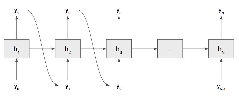
After our RNN is trained, we can use it to generate new text based on what we’ve trained it on! For example, if we trained our RNN on Shakespeare, we can generate new Shakespearean text! There are several different ways of doing this (beam search is the most popular), but we’re going to use the simplest technique called ancestral sampling. The idea is to create a probability distribution over all possible outputs, then randomly sample from that distribution. Then that sample becomes the input to the next time step, and we repeat for however long we want.

We need to pick the first character, called the seed, to start the sequence. Then, using ancestral sampling, we can generate arbitrary-length sequences! (The reason this is called ancestral sampling is because, for a particular time step, we condition on all of the inputs before that time step, i.e., its ancestors.)

In the specific case of our character model, we seed with an arbitrary character, and our model will produce a probability distribution over all characters as output. This probability distribution represents which of the characters in our corpus are most likely to appear next. Then we randomly sample from this distribution and feed in that sample as the next time step. Repeat until we get a character sequence however long we want!

But how do we create a probability distribution over the output? We can use the softmax function! Our output is essentially a vector of scores that is as long as the number of words/characters in our corpus.

$softmax(\mathbf{y})_k = \displaystyle\frac{e^{\mathbf{y}_k}}{\sum_{j=1}^M e^{\mathbf{y}_j}}$

Above, suppose our output vector has a size of $M$ . This function simply selects each component of the vector $\mathbf{y}$ , takes $e$ to the power of that component, and sums all of those up to get the denominator (a scalar). Then, we divide each component of $\mathbf{y}$ by that sum. The output is a probability distribution over all possible words/characters! Then we can sample from this distribution!

Coding an RNN

Now that we have an intuitive, theoretical understanding of RNNs, we can build an RNN! We’re going to build a character-based RNN (CharRNN) that takes a text, or corpus, and learns character-level sequences. We can use that same, trained RNN to generate text.

Let’s get started by creating a class and initializing all of our parameters, hyperparameters, and variables.

class CharRNN(object):
    def __init__(self, corpus, hidden_size=128, seq_len=25, lr=1e-3, epochs=100):
        self.corpus = corpus
        self.hidden_size = hidden_size
        self.seq_len = seq_len
        self.lr = lr
        self.epochs = epochs

        chars = list(set(corpus))
        self.data_size, self.input_size, self.output_size = len(corpus), len(chars), len(chars)
        self.char_to_num = {c:i for i,c in enumerate(chars)}
        self.num_to_char = {i:c for i,c in enumerate(chars)}

        self.h = np.zeros((self.hidden_size , 1))

        self.W_xh = np.random.randn(self.hidden_size, self.input_size) * 0.01
        self.W_hh = np.random.randn(self.hidden_size, self.hidden_size) * 0.01
        self.W_hy = np.random.randn(self.output_size, self.hidden_size) * 0.01
        self.b_h = np.zeros((self.hidden_size, 1))
        self.b_y = np.zeros((self.output_size, 1))

The corpus is the actual text input. We then create lookup dictionaries to convert from a character to a number and back. Finally, we initialize all of our weights to small, random noise and our biases to zero. Notice we also initialize our hidden state to the zero vector.

Speaking of sampling, let’s write the code to sample. Remember that we need an initial character to start with and the number of characters to generate.

def sample(self, seed, n):
    seq = []
    h = self.h

    x = np.zeros((self.input_size, 1))
    x[self.char_to_num[seed]] = 1

    for t in range(n):
        # forward pass
        h = np.tanh(np.dot(self.W_xh, x) + np.dot(self.W_hh, h) + self.b_h)
        y = np.dot(self.W_hy, h) + self.b_y
        p = np.exp(y) / np.sum(np.exp(y))

        # sample from the distribution
        seq_t = np.random.choice(range(self.input_size), p=p.ravel())

        x = np.zeros((self.input_size, 1))
        x[seq_t] = 1
        seq.append(seq_t)
    return ''.join(self.num_to_char[num] for num in seq)

Let’s suppose that all of our parameters are trained already. For a given number of time steps, we do a forward pass of the current input and create a probability distribution over the next character using softmax. Then, we randomly sample from that distribution to become our input for the next time step. We’re also recording the number so we can re-map it to a character when we print it out.

To clean up the code and help with understanding, we’re going to separate the code that trains our model from the code that computes the gradients. First, we’ll define the function to train our model since it’s simpler and help abstract the gradient computations.

def fit(self):
    smoothed_loss = -np.log(1. / self.input_size) * self.seq_len
    for e in range(self.epochs):
        for p in range(np.floor(self.data_size / self.seq_len).astype(np.int64)):
            # get a slice of data with length at most seq_len
            x = [self.char_to_num[c] for c in self.corpus[p * self.seq_len:(p + 1) * self.seq_len]]
            y = [self.char_to_num[c] for c in self.corpus[p * self.seq_len + 1:(p + 1) * self.seq_len + 1]]

            # compute loss and gradients
            loss, dW_xh, dW_hh, dW_hy, db_h, db_y = self.__loss(x, y)
            smoothed_loss = smoothed_loss * 0.99 + loss * 0.01
            if p % 1000 == 0: print('Epoch {0}, Iter {1}: Loss: {2:.4f}'.format(e+1, p, smoothed_loss))

            # SGD update
            for param, dparam in zip([self.W_xh, self.W_hh, self.W_hy, self.b_h, self.b_y], [dW_xh, dW_hh, dW_hy, db_h, db_y]):
                param += -self.lr * dparam

We smooth our loss so it doesn’t appear to be jumping around, which loss tends to do. The outermost loop simply ensures we iterate through all of the epochs. The inner loop actually splits our entire text input into chunks of our maximum sequence length. Then we convert each character into a number using our lookup dictionary. Notice that our outputs are just the inputs shifted forward by one character. It may look like we’re doing unsupervised learning, but RNNs are supervised learning models! We use a function to compute the loss and gradients. We report the smoothed loss and epoch/iteration as well. Finally, with the gradients, we can perform a gradient descent update.

Now all that’s left to do is compute the loss and gradients for a given sequence of text. Like any neural network, we do a forward pass and use backpropagation to compute the gradients.

def __loss(self, X, Y):
    xs, hs, ys, ps = {}, {}, {}, {}
    hs[-1] = np.copy(self.h)

    # forward pass
    loss = 0
    for t in range(len(X)):
        xs[t] = np.zeros((self.input_size, 1))
        xs[t][X[t]] = 1
        hs[t] = np.tanh(np.dot(self.W_xh, xs[t]) + np.dot(self.W_hh, hs[t-1]) + self.b_h)
        ys[t] = np.dot(self.W_hy, hs[t]) + self.b_y
        ps[t] = np.exp(ys[t]) / np.sum(np.exp(ys[t]))
        loss += -np.log(ps[t][Y[t], 0])

    # backward pass
    dW_xh = np.zeros_like(self.W_xh)
    dW_hh = np.zeros_like(self.W_hh)
    dW_hy = np.zeros_like(self.W_hy)
    db_h = np.zeros_like(self.b_h)
    db_y = np.zeros_like(self.b_y)
    delta = np.zeros_like(hs[0])
    for t in reversed(range(len(X))):
        dy = np.copy(ps[t])
        # backprop into y
        dy[Y[t]] -= 1
        dW_hy += np.dot(dy, hs[t].T)
        db_y += dy

        # backprop into h
        dh = np.dot(self.W_hy.T, dy) + delta
        dh_raw = (1 - hs[t] ** 2) * dh
        db_h += dh_raw
        dW_hh += np.dot(dh_raw, hs[t-1].T)
        dW_xh += np.dot(dh_raw, xs[t].T)

        # update delta
        delta = np.dot(self.W_hh.T, dh_raw)
    for dparam in [dW_xh, dW_hh, dW_hy, db_h, db_y]:
        # gradient clipping to prevent exploding gradient
        np.clip(dparam, -5, 5, out=dparam)

    # update last hidden state for sampling
    self.h = hs[len(X) - 1]
    return loss, dW_xh, dW_hh, dW_hy, db_h, db_y

The first loop simply computes the forward pass. The next loop computes all of the gradients. We didn’t derive the backpropagation rules for an RNN since they’re a bit tricky, but they’re written in code above. (We use the cross-entropy cost function, which works well for categorical data.) Additionally, we perform gradient clipping due to the exploding gradient problem.

The exploding gradient problem occurs because of how we compute backpropagation: we multiply many partial derivatives togethers. In a long product, if each term is greater than 1, then we keep multiplying large numbers together and can overflow! So we clip the gradient. Similarly, we can encounter the vanishing gradient problem if those terms are less than 1. Multiplying many numbers less than 1 produces a gradient that’s almost zero! There are more advanced and complicated RNNs that can handle vanishing gradient better than the plain RNN.

That’s all the code we need! Now we can start using it on any text corpus!

if __name__ == '__main__':
    with open('input.txt', 'r') as f:
        data = f.read()

    char_rnn = CharRNN(data, epochs=10)
    char_rnn.fit()
    print(char_rnn.sample(data[0], 100))

In the ZIP file, there’s a corpus of Shakespeare that we can train on and generate Shakespearean text! (The code we wrote is not optimized, so training may be slow!)

Below are some examples of Shakespearean text that the RNN may produce!

SEBASTIANHI:
It is flet'st and telefunture of Muckity heed.

ANTONIO:
What? Oo it is the stish is eyemy
Sseemaineds, let thou the, not spools would of
Noveit!--

ANTONIO:
Parly own ame.
Navised salied,,
It is thou may Fill flle of thee neven serally indeet asceeting wink's sabisy's corrious,
Why's, wlendy to?m.

SEBASTING:
O, speak deliaw
Thouss, for tryiely cown lest umperfions.

SEBASTIAN:
Yo af or the pauges condest I waped possitly.

SEBASTIAN:
Py himsent
Winker thy broke,
gnded when
I''stey-ingery,
My gromise!

ADNONCA:
Nothed, Goon hearts
sprair,;
And come, the Nattrevanies, as impentnems,
Who will more; senfed to make he she a kist
Is is?

ANBONIO:
&ly not friend 'rissed's poke,
To undmensen;
Nolly the purrone,!
Seo'st as inlo good nature your sweactes subour, you are you not of diem suepf thy fentle.
What you There rost e'elfuly you allsm, I-loves your goods your emper
it: seave seep. Teck:
These standly servilph allart.

ENTUSSIN:
Nay, I doce mine other we kindd, speak, yo

ure winl, funot
Show natuees
sheant-that sofe,
While y am threat,
she sills;
You more speak, you dru

 diss, it or my longly didan and to eftiscite:
My good serand
she, for yie, sir,
Can yoursely? they

Try this with other kinds of text corpa and see how well the RNN can learn the underlying language model!

Recurrent Neural Networks are neural networks that are used for sequence tasks. The flaw of previous neural networks was that they required a fixed-size input, but RNNs can operate on variable-length input! They share their parameters across sequences and are internally defined by a recurrence relation. We formulated RNNs and discussed how to train them. Finally, we wrote code for a generic character-based RNN, trained it on a Shakespeare corpus, and had it generate Shakespeare for us!

Recurrent Neural Networks are the state-of-the-art neural architecture for advanced language modeling tasks like machine translation, sentiment analysis, caption generation, and question-answering!