You can access the full course here: Bite-Sized NumPy
Table of contents
Part 1
In this lesson you will learn how to download an install Anaconda and Jupyter notebooks on your mac.
What is Anaconda?
- Anaconda is a distribution software that provides everything a user would need to start Python development.
- It includes:
- Python language
- Libraries
- Editors(Such as Jupyter Notebooks)
- Package manager
What are Jupyter Notebooks?
- A Jupyter Notebook is an open source web application that allows users to share documents with text, live code, images, and more.
- We will use this to write code as it provides an interactive and easy to use interface.
Download and Install Anaconda
Anaconda is available for download from the following link: https://www.anaconda.com/distribution/#download-section
Here is the Direct Link: Anaconda Download MAC

Once you download the file go ahead and open it, and follow the instructions in the installation wizard.
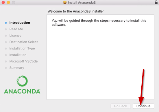
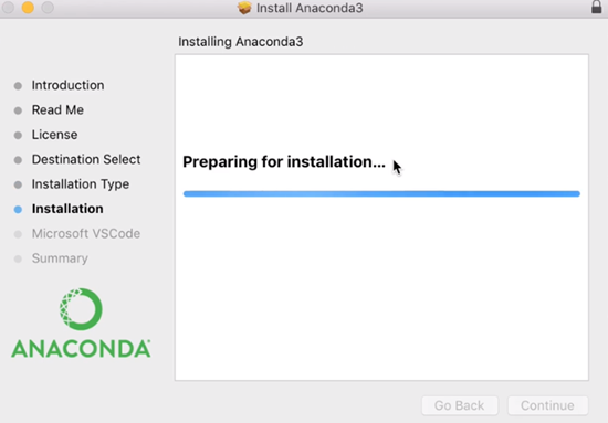
Just follow through the prompts and choose where you want to install Anaconda on your system.
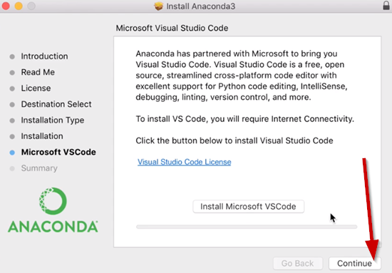
You do not need to install Microsoft Visual Code. So just hit the Continue button at that prompt.
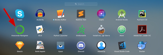
Once Anaconda is installed on your Mac system go ahead and open the Anaconda-Navigator from your applications menu.
Once Anaconda is opened it may take a view moments to initialize.
Once it’s open, you will see a few options to choose from, but we will be using the Jupyter Notebook launch button. So go ahead and select the Launch button.

Once the Juptyer Notebook loads it should look like this:
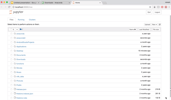
There will be a list of files and directories, and you can go to the Desktop then Jupyter Notebooks.
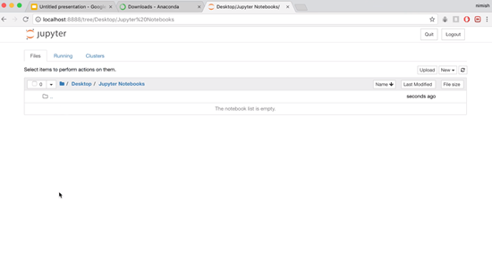
From here navigate to the New button and select Python 3.

This will open up a new Jupyter notebook and in the cells, you can write in the code.
These cells can contain text, or code. So we will choose code from the drop down menu.

So we now have Anaconda downloaded and installed for MAC.
Part 2
In this lesson you will learn how to download an install Anaconda and Jupyter notebooks on Windows.
What is Anaconda?
- Anaconda is a distribution software that provides everything a user would need to start Python development.
- It includes:
- Python language
- Libraries
- Editors(Such as Jupyter Notebooks)
- Package manager
What are Jupyter Notebooks?
- A Jupyter Notebook is an open source web application that allows users to share documents with text, live code, images, and more.
- We will use this to write code as it provides an interactive and easy to use interface.
Download and Install Anaconda
Anaconda is available for download from the following link: https://www.anaconda.com/distribution/#download-section
Here is the Direct Link: Anaconda Download Windows
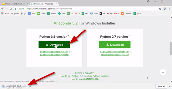
Once you download the file go ahead and open it, and follow the instructions in the installation wizard.
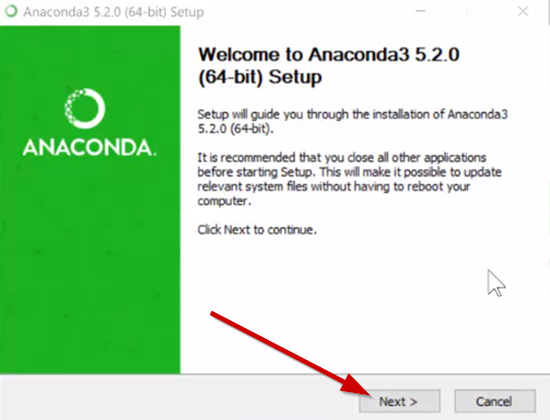
Just follow through the prompts and choose where you want to install Anaconda on your system.

You do not need to select any of the Advanced Options. So just select the Install button, but do not check any of the advanced options.
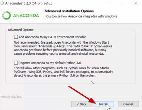
You can Skip the install of Microsoft VSCode.
Once Anaconda is installed on your Windows system go ahead and open the Anaconda-Navigator.
Once Anaconda is opened it may take a view moments to initialize.
Once its open, you will see a few options to choose from, but we will be using the Jupyter Notebook launch button. So go ahead and select the Launch button.
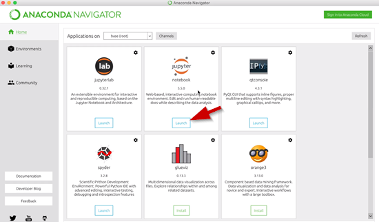
Once the Juptyer Notebook loads it should look like this:

There will be a list of files and directories, and you can go to the Desktop then Jupyter Notebooks.

From here navigate to the New button and select Python 3.

This will open up a new Jupyter notebook and in the cells, you can write in the code.
These cells can contain text, or code. So we will choose code from the drop down menu.

So we now have Anaconda downloaded and installed for Windows.
Part 3
What are Numpy Arrays?
- Numpy arrays are like lists with extra functionality
- Often used in data science and machine learning
- Very powerful with many built-in functions written in maximum efficiency
The different ways in Which Numpy Arrays can be Started:
- Pre-assigned values
- Zeroes
- Ones
- Range of vlaues
- Linspace
Open Jupyter Notebook in the Anaconda Navigator menu by selecting the Launch button.

Start a new Jupyter Notebook using Python 3.

Rename this to “Creating Numpy Array.”

We will start with the first cell being a Header so select Markdown from the drop down menu:

The Header will say “Creating Numpy Arrays”
So for starters you may have seen lists fin Python before. So in this example we will create “list1.”
See the code below and follow along:
list_1 = [1, 2, 3]
print(list_1)
So we will print this list1 and then select Run from the menu:
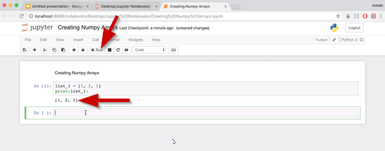
Numpy arrays are setup not so differently. Numpy arrays will take in a list as an argument and we’ll convert that list into a numpy specific array. This attaches a bunch of extra functionality to it. However before we can actually do anything we’ll want to add numpy as an import. The reason we need to do this is because numpy isn’t actually built into the native Python library. So we need to simply add the import of the numpy to cell two.
See the code below and follow along:
import numpy as np
Make sure you run cell 2.
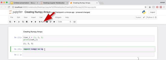
This gives us access to that library.
So let’s say we want to create a numpy based on list1 that we created in cell 1.
See the code below and follow along:
numpy_1 = np.array(list_1)
print(numpy_1)
Run the cell.

We again got 1, 2, 3 printed out just like before.
You will notice the format is a little different.
The first cell was a list but the third cell was a numpy array. Earlier, it was mentioned that we can create arrays of zeroes or ones. This is very often a starting point for such topics as machine learning. Like if you were to build machine learning software, and we know that we want an array maybe of size 20. So we want 20 elements in an array. We might initialize the array to be 20-zeroes or 20-ones. Then we can go and modify each element.
So the way in which we do this is by calling the zeroes or the ones operator. So we could create for example a zeroes array. See the code below and follow along:
zeros_array = np.zeros(5)
print(zeros_array)
Run the cell.

So we get an array of five zeroes.
We can do the same thing for ones. See the code below and follow along:
ones_array = np.ones(10)
print(ones_array)
Run the cell.
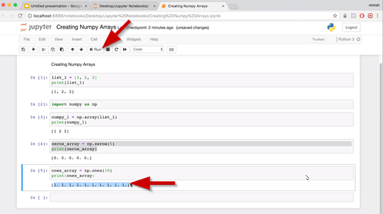
So we have the array of ones that was printed out for us.
So if we wanted maybe a start point and an end point, and add a step interval. See the code below and follow along:
range_array_1 = np.arange(5)
print(range_array_1)
Run the cell.
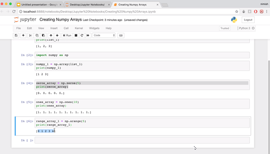
So we get five elements printed out, but this might not be what we expected, because we put in a “5” with the “arange” operator this is the upper bound. So this is saying its going to stop before it reaches five. We were only specifying the end point.
So if we want to specify a start point as well, let’s say we want the elements five to 10. See the code below and follow along:
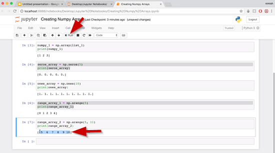
range_array_2 = np.arange(5, 11)
print(range_array_2)
Run the cell.
Now let’s say we want to step by twos. So maybe we want to start at zero go until 20 and we want to skip every other element. We can do that be specifying a third parameter being the step. See the code below and follow along:
range_array_3 = np.arange(0, 20, 2)
print(range_array_3)
Run the cell.

The final thing we will cover is the linspace operator. Linspace is a conjunction for linear space. With the linspace we basically take a lower bound an upper bound and the number of elements we want it to populate between the upper bound and lower bound. See the code below and follow along:
linspace_array = np.linspace(0, 10, 5)
print(linspace_array)
Run the cell.
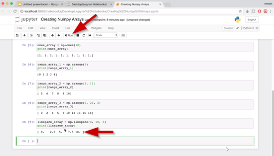
So what this has done is created an array of five elements evenly spaced between zero and ten. Again ten inclusive, zero inclusive.
This will be really useful to us when it comes to graphing values. Because we can just specify and upper bound and a lower bound and then how many points we want in between those two.
That’s it for this NumPy tutorial. If you want to check out more, you can try the free video below to gain further insight into the power of NumPy. Then, jump into our Data Science Mini-Degree to gain further skills!
Transcript 1
We’ll simply search for download Anaconda, and we’ll want to select this first link here, this is conda.io. So what we wanna do is download Anaconda here, so we’ll click on this link and this brings us to the Anaconda website.
So there’s a couple of options to choose from depending on whether you’re using Mac, Windows, or Linux. So, we’ll just simply click on this link (unless you really want Python 2.7). I would actually recommend that you use Python 3.6 anyway. So, we’re gonna go ahead and download this. By the way, if you are using a PC, then actually feel free to skip to the next section. We’ll be showing you the same stuff for PC.
Alright, so it looks like that’s finished downloading. We’ll simply double click on this, and it should bring up an installation wizard. So let’s go and bring up the installer. So, we’ll just go ahead and continue. Alright, so it just took a few minutes, and it’s done now. We’re not gonna bother installing Microsoft Visual Studio Code or anything like that, so let’s not worry. We’ll just continue and go ahead and close this; we can simply move that installer to trash.
Okay, so now what we’ll want to do is just go into our applications, and you should see Anaconda-Navigator. So, we are going to select this guy here. There are a few options to choose from, but we’ll definitely want Jupyter notebook here. This is version 5.5.0 at this time. So let’s go ahead and actually just launch this. What this’ll do is start a new instance of Terminal, and actually, weirdly enough, we can go to the Terminal itself and just type Jupyter notebook, and we’ll start notebook that way, but we might as well use Anaconda. It’s a nice piece of software to use anyway.
So as you can see here, this actually brings up a list of a bunch of my files and directories. So what we’re gonna do is actually go to Desktop here. This is just my file system on my computer, and we’re just gonna go into Jupyter Notebooks. So from here, I can simply select a new notebook. I’m going to go for Python 3. Otherwise, you could do like Text File, Folder, Terminal. What we’ll actually want is a Python 3 notebook.
This now opens up a new Jupyter notebook and a new tab here, and if we navigate back here, you can see that there is a new notebook IPYNB. This is a Jupyter notebook here. Now, we haven’t given it a name. This is running right now so we can go ahead and give this a name if we want up here. And then, we will just write a code in these little cells. So these cells can contain text or code which have we choose. We can choose Code, Markdown, NBConvert, or Heading. Typically, we’ll just go with Markdown for regular text, and we’ll just write- but we’ll choose the Code one for some Python code that we can actually write and run.
So let’s say for example, we just wanted to actually just print out a variable. I could create a variable code like int1 and I could set this equal to five, and then I could print int1. Okay, If I go to “Run this Cell”, then it simply runs all of the code that’s in this particular cell and starts a new one.
Transcript 2
Anaconda downloads page. If you’re not sure where to find this, then you can simply search for Download Anaconda. Okay, we’ll go to this first one. Then, we’re going to go down to Download Anaconda for free, and it should take you right to that page here. So what we’ll want is the Windows Installer, so let’s go ahead and select that. I would recommend going with the later version 3.6, as there are a bunch of tools that aren’t included in 2.7. If you’re really dead set on 2.7 you can use that, but I would, again, recommend 3.6.
So let’s just go ahead and download that, and I’m just gonna actually pause the recording on my end and cut back once this is done.
Alright, and we are back. So it finally finished downloading (it took a few minutes), and I just opened up the executable file. Alright, and it looks like we’re finally done with the installation, so let’s just go ahead and finish this off. We’re gonna skip this, we don’t really want to install Microsoft Visual Studio code right now. We’ll just uncheck these boxes, unless you do indeed want to learn more about these.
So let’s go ahead and finish that up, and now let’s open up Anaconda, start a new Jupyter notebook, and then I’ll just really quickly explain what they’re all about. So we’re just gonna search for Anaconda, and we’ll want this guy here, the Anaconda Navigator. So let’s just go ahead and select it, and we’re gonna go for a Jupyter notebook here. So let’s launch that up, and it will launch a new directory kinda thing in the browser here.
As you can see, it says home and gives us a list of files and directories in the directory that Anaconda is saved in. Okay, so what we’re gonna do for now is just navigate to the correct directory that you want, and we’re just gonna select a new Python 3 notebook. So what this’ll do is it’ll start a new Jupyter notebook. This is what a default one looks like; you can give it a title by clicking up here, and there’s a few options to choose from as far as actions go. You can see that there’s this cell here, and the way Jupyter notebooks work is that basically we write and run code in individual cells. That being said, the code that we write in one cell persists into the next cell.
Let’s say, for example, I’m just gonna create a quick markdown just to show you what this is. It’s just to hold some text, so it’s kind of like a text holder. Okay, we run this cell to complete it, okay? Because this is just text, there’s nothing to run. But let’s say I created a variable called variable one, I set its value equal to five, I run this, and unless there’s a problem with the code, it should compile and run just fine. Now if I go to print variable one, that code should persist between the cells, so if I run this, it will execute the code found here, and it will start me a new cell.
That’s how Jupyter notebooks work. It’s a really nice, clean way to organize things into individual cells.
Transcript 3
Okay, so for starters, you might have seen lists in Python before. For example, we could create list_1, we go to “Run the Cell”, we just get the simple array.
Well NumPy arrays are set up not so differently, so we’ll simply add the import of NumPy. We can also rename this to np as you’ll often see. So we’ll go ahead and run that cell. Nothing exciting happened because we’re not printing or calculating anything, we’re just gaining access to that library.
So let’s say I want to create a NumPy based on my list_1. So I’m gonna call this numpy_1. This is just going to actually be equal to np.array, and then we can pass in whatever value we want. So we could pass in a list of values here, or we could actually pass in a pre-made list. In our case, maybe we want to pass in list_1 and then perhaps we’ll want to print out numpy_1. So let’s go ahead and save that, and if we were to run the cell, we would again get one, two, three printed out just like before.
Now as I mentioned earlier we can also create arrays of zeros or ones. This is going to be np- not array this time- but np.zeroes. Now zeroes actually takes in an argument, and it takes in how many elements we want in this array. So say we want five zeroes here, and then we want to perhaps print out a zeroes array. And if we were to run this cell an array of five zeroes here. Again, we could do the same thing for one, and we’ll print this out, and then, of course, the array of ones here.
But what if we want to specify a range of values so we want maybe a start point and an endpoint? Np dot, and we’re gonna use this arange operator, operation rather, and this can take in several different parameters. So if we want to just specify a range from zero to some value, maybe let’s say zero to five, we can enter that. Okay, and as you can see we get five elements printed out. So if we want to specify a start point as well, let’s say we want the elements five to 10 and we’re going to set np.arange from five up until, and if we want to include 10, we would have to put up until 11. So now we go to run the cell, we get five, six, seven, eight, nine and 10 printed out.
Now let’s say we want to step by twos, so we want to maybe start at zero, go until 20 and we want to skip every other element. Well we can do that simply by specifying a third parameter, being the step zero to 20, and then we’ll want to include the step of two. So let’s go ahead and run that cell. And we get exactly what we would want here.
So linspace is a conjunction for linear space, and with a linspace we basically take a lower bound, an upper bound, and the number of elements we want it to populate between that upper bound and lower bound. This is going to be np.linspace like this, okay? And we’ll need to provide some parameters. So the first will be the lower bound. Let’s actually just go from zero. The second will be the upper bound. Let’s go to 10. So let’s see if we just pass in the value of five and then go to print. So we get zero, 2.5, five, 7.5, and 10. So what this has done is it’s basically created an array of five elements, evenly spaced between zero and 10, and again, 10 inclusive, zero inclusive.
Interested in continuing? Check out the full Bite-Sized NumPy course, which is part of our Bite-Sized Coding Academy.


